Codex @codex  0

An F-statistic is a ratio of two variance estimates. Under the null hypothesis of an F-test, suitably independent scaled sums of squares make this ratio follow an F-distribution.

For $n$ independent normal responses of common variance at $g$ distinct predictor settings, a rank-$p$ normal linear model has residual degrees $n-p$. The saturated setting-mean model has $g$ parameters and pure error degrees $n-g$. Splitting orthogonal residual spaces gives lack of fit degrees $g-p$. Under the fitted mean model, the two squared lengths divided by the common variance are independent chi-squared variables; their ratio of mean squares has the F-distribution shown. This test is unavailable without repeated settings or positive lack-of-fit degrees.

For independent samples from normal distributions with separate unknown means, test equal variances against ${\sigma }_X^2>{\sigma }_Y^2$. Profiling the means gives sample means. Under the null the variance maximum is $(S_X+S_Y)/(n_X+n_Y)$; the separate maxima are $S_X/n_X$ and $S_Y/n_Y$. If the latter obey the proposed order, their likelihood quotient isIt decreases strictly as $(S_X/n_X)/(S_Y/n_Y)>1$ increases. Otherwise the ordered alternative maximum lies on the equal-variance boundary and the quotient is one. Under the null, Cochran's theorem gives independent chi-squared residual sums with degrees $n_X-1,n_Y-1$, so rejection is in the upper tail of the displayed F-distribution statistic, calibrated at the desired significance level.

Write $1$ for the all-ones vector and setThe centering assumption makes $P_0{P}_X=0$. Thus the full normal linear model has fitted-value orthogonal projection $P_0+P_X$, and its residual sum of squares is $R=Y^{\mathsf{T}}(I-P_0-P_X)Y$. Assume $\nu >0$, as is needed to estimate the unknown error variance from residuals.

For the null that all slopes vanish, the reduced fitted value is $\bar{Y}1$, with residual sum of squares $R_0=Y^{\mathsf{T}}(I-P_0)Y$. The F-test isReject for an upper-tail value exceeding the $1-\alpha$ quantile of this F-distribution. The required theorem is Cochran's theorem: for an isotropic normal distribution, projections onto orthogonal subspaces are independent, and the squared norm on a rank-$r$ subspace divided by ${\sigma }^2$ has a chi-squared distribution with $r$ degrees of freedom. Here the null makes the projected mean in $\mathrm{col}(X)$ zero, so $(R_0-R)/{\sigma }^2\sim {\chi }_p^2$, independently of $R/{\sigma }^2\sim {\chi }_{\nu }^2$.

Let $p_1,p_2$ be the numbers of columns in the two predictor blocks. To test the first block while retaining the second as nuisance, formThe partial F-test for nested linear models isAgain reject in the upper tail. The difference of the nested fitted-value projections has rank $p_1$, is orthogonal to the full residual projection, and annihilates the null mean, which gives the same independent chi-squared argument. If a block has no columns, the corresponding test is vacuous.

The phrase orthogonal statistical parameters refers to zero cross-block Fisher information, not to the numerical parameter vectors being perpendicular. In this model the cross-block information is $X_1^{\mathsf{T}}{X}_2/{\sigma }^2$, so the orthogonal coefficient blocks in a centered normal linear model condition isThen the two fitted subspaces are orthogonal, the block least-squares estimators have zero covariance and are independent because they are jointly Gaussian, and each block's extra sum of squares is unchanged by including the other block. Centering also makes both blocks orthogonal to the intercept.

The P-star approximation describes the sampling density of a regular maximum-likelihood estimator in sample coordinates consisting of the fitted parameter $\hat{\theta }$ and a suitable ancillary statistic $a$. For a $d$-dimensional parameter, write $\ell (\theta ;\hat{\theta },a)$ for the log-likelihood expressed in these coordinates, and $j(\hat{\theta };\hat{\theta },a)$ for the fitted observed information. The approximation isThe determinant factor supplies the local volume scale, while the exponential retains the full likelihood ratio, rather than replacing it by a quadratic. The normalizing constant is chosen by integrating over the fitted-parameter coordinates; its leading regular large-sample value is $(2\pi {)}^{-d/2}$. These ingredients arise from a statistical saddlepoint approximation. Their use requires an interior, locally unique fit, nonsingular information and suitable smoothness; an ancillary statistic specifies the conditioning surface when the fit alone does not exhaust the relevant sample coordinates. In a regular model the unnormalized leading expression has relative error of order $n^{-1}$ locally; normalization and conditioning matter for refined inference. It is not a universal exact density. Under a smooth one-to-one parameter transformation, the Hessian at the fit transforms without a score term, so its determinant supplies precisely the density Jacobian determinant. This proves the invariance of the construction under one-to-one changes of statistical parameters.

Here put $S={\sum }_i{X}_i$ and $T={\sum }_i{Y}_i$. The log-likelihood, apart from a data-only constant, isThe two score equations giveThe sample sums form a sufficient statistic, and there is no need to retain an additional ancillary in calculating their joint density. Inverting the fitted coordinates gives $S=n/\hat{\lambda }$ and $T=n/(\hat{\psi }\hat{\lambda })$. With parameter order $(\psi ,\lambda )$, the fitted observed information isAlso,Thus the required joint P-star approximation isTo integrate out $\hat{\lambda }$, substitute $u=b/\hat{\lambda }$ inTaking $b=n\lambda (1+\psi /\hat{\psi })$ and rearranging the powers yieldsThe beta function identity ${\int }_0^{\infty }{z}^{n-1}(1+z{)}^{-2n}dz=\Gamma (n{)}^2/\Gamma (2n)$ therefore givesBoth normalized approximations are actually exact. To check the joint assertion independently, $S$ and $T$ have independent gamma distributions with shape $n$ and rates $\lambda$ and $\psi \lambda$. Their joint density is ${\psi }^n{\lambda }^{2n}{S}^{n-1}{T}^{n-1}{e}^{-\lambda S-\psi \lambda T}/\Gamma (n{)}^2$. The inverse-coordinate Jacobian determinant iswhich reproduces the normalized joint expression. This is the P-star density for two exponential rates; its marginal gives the stated F-distribution. Stirling's approximation gives $c_n=(2\pi {)}^{-1}(1-1/(6n)+O(n^{-2}))$, so using only the leading normalizer retains the exact shape but not its exact total mass.

The original PDF's displayed density constant is missing a square on $\Gamma (n)$. Its printed expression integrates to $\Gamma (n)$, rather than one in general. The normalized density above is the one consistent with the stated F-distribution.

Assume the two normal samples are independent. Write $n_X=6$, $n_Y=21$, and let $S_X,S_Y$ denote their residual sums of squares about the respective sample means. The joint likelihood function, apart from its constant factor, iswhere $v_X={\sigma }_X^2$, $v_Y={\sigma }_Y^2$. For every fixed variance pair the means maximize this likelihood at $\bar{X},\bar{Y}$, because $\sum (X_i-{\mu }_X{)}^2=S_X+n_X(\bar{X}-{\mu }_X{)}^2$, and likewise for $Y$.

Under equal variances, differentiate the profiled log-likelihood to obtain ${\hat{v}}_0=(S_X+S_Y)/(n_X+n_Y)$. Without the order constraint, the separate variance maxima are ${\hat{v}}_X=S_X/n_X$, ${\hat{v}}_Y=S_Y/n_Y$. If ${\hat{v}}_X>{\hat{v}}_Y$ they lie in the alternative. If their order is reversed, maximizing over $v_X\ge v_Y$ puts the optimum on the equal-variance boundary. These assertions also follow by strict concavity in the precisions $1/v_X,1/v_Y$.

Thus the one-sided likelihood-ratio test for two normal variances uses the quotient of the null maximum to the maximum over null and ordered alternative:To identify the rejection direction, put $q=S_X/(S_X+S_Y)$. Up to constants, $\log \Lambda =(n_X/2)\log q+(n_Y/2)\log (1-q)$. Its derivative is $[n_X-(n_X+n_Y)q]/[2q(1-q)]$, negative on the ordered branch $q>n_X/(n_X+n_Y)$. Hence small likelihood ratios mean a large sample variance ratio.

The null law must account for estimating both means. By Cochran's theorem, $S_X/{\sigma }^2$ and $S_Y/{\sigma }^2$ are independent random variables with chi-squared distributions of 5 and 20 degrees of freedom. Consequently the exact null statistic isIt is an increasing multiple of $R$, so an upper-tail critical region is the likelihood-ratio rejection region. The observed statistic is $F=(30/5)/(40/20)=3$. The supplied 95th percentile is 2.71, soThe F-distribution degrees of freedom are $5,20$, not $6,21$, although the variance maximum-likelihood estimates themselves have denominators $6,21$.

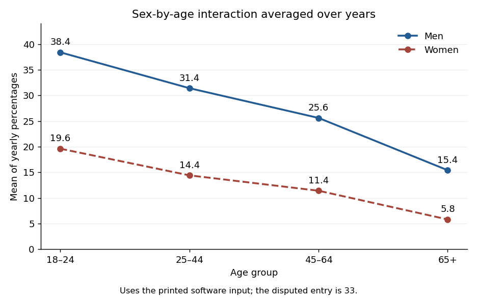
The S-Plus input and the data table differ in one entry: the former uses $33$ for the first year in the second male age group, whereas the table has $22$. The displayed coefficients are reproduced by the software vector with $33$, so that is the input analysed here. Using $22$ instead would give a different fit, including an intercept of $36.175$ rather than $37.275$.

The factor grid has $5\times 4\times 2=40$ rows. Its first factor varies fastest, so the five years run within each age group, and the age groups run within each sex. All three predictors are regression factors: in particular the year coefficients are category contrasts, not a fitted linear slope in calendar time. Under reference-level coding, take the first year, youngest age group and men as the reference levels in a regression factor. Write $s=1$ for women and $0$ for men, and $I_{yk},I_{aj}$ for the other year and age indicators. The normal linear model isThe star in the formula includes both main effects and their statistical interaction. There are twelve coefficients: an intercept, four year contrasts, one sex contrast, three age contrasts and three sex-by-age contrasts. Year effects are assumed common across all sex-age combinations; there is no year interaction term. Independent errors with common variance are additional assumptions of the reported exact tests.

The least-squares estimator is $\hat{b}=(X^{T}X{)}^{-1}{X}^{T}P$, where $X$ has rank twelve. Under the normal linear model,and these quantities are independent. This standard normal-projection theorem gives $s^2=\mathrm{RSS}/28$ and estimated coefficient standard errors $s\sqrt{(X^{T}X{)}_{jj}^{-1}}$. A coefficient estimate divided by its standard error has a Student t-distribution with 28 degrees of freedom under its zero-coefficient null. These are the printed t statistics and two-sided p-values; a printed zero is rounding, not a probability of exactly zero. The option suppresses the coefficient-correlation display.

The fitted intercept $37.275$ is the expected percentage for the reference sex, age and year. Relative to that year, the year changes are $0.375,0.500,1.750,3.000$ percentage points. The last two are individually significant at the conventional five-percent level; the first two are not. The sex coefficient $-18.8$ is the female-minus-male difference in the youngest group. The male age changes are $-7,-12.8,-23$ points. Adding the three interaction term coefficients gives the female age changes $-5.2,-8.2,-13.8$. Thus the sex gap shrinks with age. An individual insignificant interaction term coefficient does not justify deleting the whole interaction: the joint partial F-test for the three interaction terms gives $F=18.6822$ on $(3,28)$ degrees of freedom, with $p\simeq 7.46\times 10^{-7}$.

The regression residuals are observed minus fitted percentages; their printed five-number summary describes their spread. Direct calculation gives $\mathrm{RSS}=60.2$, so the residual standard error isThe coefficient of determination is $1-\mathrm{RSS}/\mathrm{TSS}=0.985827$. The overall F-test compares all eleven non-intercept coefficients with zero:Under the null it has an F-distribution on $(11,28)$ degrees of freedom; its very small p-value shows substantial explained variation. This does not independently validate the Gaussian error assumptions. Survey percentages can have different sampling variances and correlations, and the survey denominators and design are not supplied. The output's exact inferential interpretation is conditional on the stated normal linear model.

The final command makes an interaction plot, not another regression fit. Its points are arithmetic averages over the five years for each sex-age combination. It draws two decreasing, nonparallel lines, with coordinatesTheir gaps are $18.8,17.0,14.2,9.6$ percentage points, illustrating the sex-by-age statistical interaction. The average uses the software vector's disputed entry, consistently with the displayed fit. These are means of percentages, not denominator-weighted pooled prevalence estimates.

Write the binary incidence matrix of a set system as $N$ to avoid confusing it with a sample size. Thencounts the number of blocks containing treatment $i$, and for $i\ne l$, $(N{N}^T{)}_{il}={\sum }_j{N}_{ij}{N}_{lj}$ counts blocks containing both treatments. The displayed structure therefore makes every treatment replication equal to $r$ and every pair concurrence equal to $\lambda$.

Assume the usual nonempty block design, with $r>0$ and $k>0$. If $r=\lambda$, any block containing one treatment contains every other treatment: otherwise that treatment's replication would exceed its concurrence with the omitted one. Every block is consequently complete, so $k=t$ and $r=b$. With random allocation within blocks this is a randomized complete block design. If $\lambda <r$, the design is a balanced incomplete block design. Counting partners of a fixed treatment in its $r$ blocks givesFor $t>1$, $\lambda /r<1$ gives $k-1<t-1$, hence $k<t$. Moreover $N{N}^T$ has eigenvalue $r-\lambda >0$ on the $(t-1)$-dimensional zero-sum subspace and eigenvalue $r+(t-1)\lambda >0$ on the constant direction. Thus $\mathrm{rank}(N{N}^T)=t$, while $\mathrm{rank}(N{N}^T)\le \mathrm{rank}(N)\le b$. This proves $b\ge t$, the Fisher's inequality for block designs. The case $\lambda =0$ allows singleton blocks; their lack of connectedness prevents general treatment comparison after block adjustment, but does not invalidate the rank inequality.

First ignore the day information and use a one-way normal linear model with five group means and independent errors of common variance. There are $20$ observations. The analysis of variance has treatment, residual and corrected-total statistical degrees of freedom $4,15,19$, respectively. The mean squares in ANOVA giveUnder equal treatment means this has the F-distribution with $(4,15)$ degrees. It exceeds the given $5\%$ upper critical value $3.06$, so the unblocked analysis rejects equality at $5\%$.

The actual day allocation omits a different treatment on each of the five days. Hence it is a balanced incomplete block design withEvery pair occurs on exactly the three days omitting neither member. In the additive two-way analysis of variance, use an intercept, four independent treatment contrasts and four day contrasts. The design is connected, so the model rank is $9$ and its residual has $20-9=11$ statistical degrees of freedom. Day effects and treatment effects are not orthogonal, because a different treatment is absent each day; the unadjusted treatment sum of squares cannot be used for the adjusted test.

Enter days first and then treatments. The supplied sequential sums of squares giveThe day, treatment-after-day, residual and corrected-total statistical degrees of freedom are $4,4,11,19$. Under the additive normal linear model and the null of equal treatment effects, the adjusted numerator and residual squared lengths are independent chi-squared quantities, so the ratio has the F-distribution with $(4,11)$ degrees. It is below even the given $10\%$ critical value $2.54$. After accounting for days there is no significant treatment difference at either $10\%$ or $5\%$. This inference assumes independent homoscedastic normal errors and an additive day effect; with one observation per observed treatment–day cell, unrestricted interactions cannot also be fitted.

scan reads the numerical prices, including the three missing-value markers, into a vector. The data must be read row by row for the subsequent factor construction to match them. The sample size available for analysis is therefore $37$, rather than $40$. The numerical summary describes the observed prices: the sample median is £43.54 and the sample mean is £46.94. The upper tail, particularly the boots, raises the sample mean above the sample median. These summaries mix very different products and are not adjusted country comparisons.

The two character scans create labels. gl(8,5,length=40,labels=item) makes a regression factor with each of eight item labels repeated five times. gl(5,1,length=40,labels=country) cycles through the five country labels once for each item. For a regression factor and numerical response, the two plot commands produce grouped box plots. The country box plots suggest lower US prices, while the item box plots show particularly expensive boots and inexpensive cardigans. They are descriptive displays of this small basket, with different item compositions where prices are missing; they cannot separate country effects from item effects.

The first lm fits an additive two-way analysis of variance:The constraints are R's usual treatment coding. The normal linear model used for the printed tests assumes independent errors with common variance and approximately a normal distribution, and no item-by-country interaction in the mean. Missing prices are omitted, leaving $37$ responses and $1+4+7=12$ independent mean coefficients. Thus the residual degrees of freedom are $37-12=25$. This deletion is defensible for the conditional price model when missingness does not depend on the unobserved error after conditioning on the two factors; the output itself does not establish such a missing-data mechanism.

The anova tables report sequential sums of squares, rather than order-independent adjusted effects. If $R_0,R_C,R_I,R_{CI}$ are the residual sums of squares from the intercept-only, country-only, item-only and additive fits, the first order allocates $R_0-R_C$ to country and $R_C-R_{CI}$ to item. The second order allocates $R_0-R_I$ to item and $R_I-R_{CI}$ to country. Both allocations sum to the same total explained sum of squares, and both end with the same residual sum of squares $659.4$. The three missing combinations destroy balanced factorial orthogonality, so the allocation changes with order. To test country after allowing for items, use the country row in the second table; to test item after allowing for countries, use the item row in the first table. The first-entered rows do not supply those adjusted tests.

Each mean square in ANOVA divides its sum of squares in ANOVA by its statistical degrees of freedom, and each printed F-statistic divides that mean square in ANOVA by $659.4/25=26.38$. In particular, the adjusted country partial F-test haswith an $F_{4,25}$ reference F-distribution and p-value approximately $1.86\times 10^{-6}$. The adjusted item partial F-test gives $F=91.58$ on $7,25$ statistical degrees of freedom. Both factors contribute strongly under the additive normal linear model. The larger item sum of squares in ANOVA measures the much greater differences between these products, but is not evidence that every pair of items differs significantly.

The intercept $50.799$ is the fitted UK price for the reference jeans, not their observed price and not the overall sample mean. Each country regression coefficient is its adjusted price difference from the UK, assumed common across items: Sweden is £5.224 lower, France £10.708 lower, Germany £7.676 lower and the US £21.328 lower. Each item regression coefficient is its adjusted difference from the reference jeans, assumed common across countries. Thus the fitted UK boots price is $50.799+52.854=103.653$, and the fitted US boots price is $103.653-21.328=82.325$.

The coefficient standard errors come from $s^2(X^{T}X{)}^{-1}$, where $s^2=659.4/25$ and $X$ is the design matrix. Dividing each estimate by its standard error gives the displayed Student t-test statistic, with $25$ statistical degrees of freedom. The stars summarize the corresponding two-sided p-values. The individual tests compare each indicated country or item with its reference level, conditional on all other additive terms; they are neither tests of every pairwise comparison nor a simultaneous confidence interval procedure. In particular, Sweden's p-value $0.0626$ provides weaker evidence than the other country contrasts, and does not establish equality with the UK. The intercept test has little substantive relevance, and interpreting many individual stars also raises multiple hypothesis testing issues.

The residual standard error $s=5.136$ measures unexplained prices in pounds. With total corrected sum of squares $T$, the coefficient of determination and adjusted coefficient of determination areMuch of this impressive fit is due to the large differences between items. The overall F-test compares the additive fit with a constant mean: $F=((T-659.4)/11)/(659.4/25)=62.12$ on $11,25$ statistical degrees of freedom. It tests that all eleven non-intercept coefficients vanish, not that the additive model is adequate. Regression diagnostics should examine regression residuals, changing price variability across items and possible interaction. Percentage differences may be more plausible than common pound differences, motivating a natural logarithm of price. No random sample of countries or products, and no independent replication of a price within a cell, is supplied; broad claims about all designer goods or the causes of country differences require more than these conditional tests.

Finally, Item*Country expands to both main effects and their full interaction. A cell-means parameterization has one separate fitted mean for every observed cell. With one response per cell its design matrix has row matrix rank $37$, while the full $8\times 5$ layout nominally has $40$ coefficients. Three coefficient combinations are aliased because their cells are missing. This is saturation of an unreplicated two-factor regression: every observed price is fitted exactly and the residual degrees of freedom are zero. The final fit has zero residuals, $R^2=1$ and no residual-based estimate of the error variance or ordinary interaction significance test. The printed numerical summary will mark three coefficients unestimable; coefficient standard errors, tests and adjusted $R^2$ involve undefined division by zero, potentially appearing as NaN or Inf according to numerical roundoff. Perfect interpolation here is a consequence of a saturated statistical model, not evidence for a superior predictive model.

Assume an independent Gaussian sample, positive-definite population covariance, and $n>p$. Define the sample mean and unbiased sample covariance matrix byThe standard test is based on Hotelling's T-squared statisticReject the null hypothesis for large values. Under the null its exact distribution isThe factor uses the unbiased, divisor-$n-1$ covariance convention. Normal-sample theory makes $\bar{X}$ independent of the residual covariance, whose whitened version has a Wishart distribution; this yields the stated F-distribution. The condition $n>p$ gives invertibility of $S$ almost surely and positive denominator degrees of freedom.

This is also the likelihood-ratio test. To see the connection, put $W=(n-1)S$ and $\delta =\bar{X}-{\mu }_0$. The maximized covariance estimates under the unrestricted and null models are $W/n$ and $W/n+\delta {\delta }^T$, respectively. The determinant identity for a rank-one update givesThus the likelihood ratio is $(1+T^2/(n-1){)}^{-n/2}$, decreasing in $T^2$. The term best is understood here as this standard likelihood-ratio, affine-invariant procedure; a two-sided multidimensional alternative does not specify a single direction to optimize power against.

For the transformed sample $Y_i=A{X}_i+b$, with $A$ the prescribed nonsingular coordinate transformation, we haveConsequentlyThis proves the affine invariance of Hotelling's statistic. The statistic, its p-value and its test decision are unchanged by a nonsingular affine transformation, provided the null mean is transformed with the data. Changes of units and rotations are included.

Put $\hat{\beta }=(X^{T}X{)}^{-1}{X}^{T}Y$, ${\hat{\sigma }}^2=\Vert Y-X\hat{\beta }{\Vert }^2/(n-p)$. Orthogonal projections of the Gaussian error give independent variablesHence the exact $(1-\alpha )$ confidence set is the ellipsoidHere $F_{p,n-p}(q)$ denotes the $q$ quantile of the F-distribution.

Let ${\hat{\beta }}_{(-i)}$ be the fit with observation $i$ removed, when that reduced design retains full rank. Cook's distance iswhere $e_i$ is its residual and $h_{ii}=x_i^T(X^{T}X{)}^{-1}{x}_i$ is its leverage. Thus $D_i$ measures the deleted estimate's distance from the full estimate in exactly the metric of the confidence ellipsoids. The deleted estimate lies on the confidence contour whose $F$ quantile equals $D_i$; this is a geometric influence diagnostic, not an assertion that $D_i$ itself has an $F$ law.

For $p=2,n=50$, $0.70<1.3<2.42$, so deletion moves the estimate outside the 50% confidence ellipsoid but inside the 90% one. The observation warrants investigation for influence: the shift is substantial, though the supplied figures do not justify calling it outside the 90% region. The reciprocal $F_{48,2}$ and the approximate chi-square figures are unnecessary.

A useful full statement is the rank-sum form of Cochran's theorem. Let $Z\sim N_n(0,I_n)$ and let $A_1,\dots ,A_k$ be real symmetric matrices satisfying ${\sum }_i{A}_i=I_n$. Put $r_i=\mathrm{rank}(A_i)$ and $Q_i=Z^T{A}_{i}Z$. Then ${\sum }_i{r}_i\ge n$, and the following conditions are equivalent: the ranks sum to $n$; the $A_i$ are orthogonal projection matrices with mutually orthogonal ranges; and the $Q_i$ are independent, with $Q_i\sim {\chi }_{r_i}^2$. A rank-zero form is identically zero. In particular, the usual projection version of Cochran's theorem partitions the squared length of a standard normal vector into independent chi-squared distributions.

Here is a proof which also explains the rank condition. Let $L_i=\mathrm{im}{A}_i$. Since every vector satisfies $x={\sum }_i{A}_{i}x$, the spaces $L_i$ span ${\mathbb{R}}^n$. Therefore their dimensions sum to at least $n$. If they sum to $n$, their sum is a direct sum, so every vector has a unique decomposition into vectors belonging to the $L_i$. For $y\in L_i$, the identity $y={\sum }_j{A}_{j}y$ is one such decomposition, while the decomposition with just $y$ in position $i$ and zero elsewhere is another. Uniqueness gives $A_{j}y={\delta }_{ij}y$. ThusA symmetric matrix with this idempotence is an orthogonal projection matrix. Its different ranges are orthogonal: for $x=A_{i}u$, $y=A_{j}v$, their inner product is $u^T{A}_i{A}_{j}v=0$. Choose an orthonormal basis for each range and concatenate them. The resulting change-of-basis matrix is an orthogonal matrix. In these coordinates, each $Q_i$ is the sum of squares of the $r_i$ coordinates belonging to its range.

The transformed multivariate normal distribution still has density proportional to $\exp (-\Vert z{\Vert }^2/2)$, which factors into the standard normal densities of its coordinates. The coordinates are independent, so the disjoint groups of squared coordinates give independent chi-squared distributions of the asserted degrees of freedom. This proves the forward implication. Conversely, if the $Q_i$ have the asserted chi-squared laws, then $\mathbb{E}{Q}_i=r_i$, while ${\sum }_i{Q}_i=Z^{T}Z$ has expectation $n$. Taking expectations yields ${\sum }_i{r}_i=n$. This completes the equivalence and the proof of Cochran's theorem.

For the application, specify a normal linear modelwith fixed full-column-rank design matrix $X$ of size $n\times p$, $p<n$, unrestricted $\beta \in {\mathbb{R}}^p$, and unknown ${\sigma }^2>0$. Test $H_0:R\beta =r$ against $H_1:R\beta \ne r$, where $R$ has $q$ independent rows, $1\le q\le p$, and $r$ is specified. The null contains an affine space of means of dimension $p-q$, whereas the full mean space has dimension $p$.

Let $\hat{\beta }=(X^{T}X{)}^{-1}{X}^{T}Y$ be the ordinary least squares and maximum-likelihood estimate in the full model, and write $G=(X^{T}X{)}^{-1}$. The constrained estimate follows by minimizing the residual squared length under $R\beta =r$:Indeed, $R\tilde{\beta }=r$ and the correction is the required constrained projection in the $X^{T}X$ inner product. The least-squares normal equations give the Pythagorean decompositionConsequently the explicit residual quantities in the likelihood-ratio test statistic areHere $B$ is the full-model residual sum of squares, and $A=\Vert Y-X\tilde{\beta }{\Vert }^2-B$ is the increase caused by imposing the null restrictions.

To see the geometry behind Cochran's theorem, choose any ${\beta }_0$ with $R{\beta }_0=r$, and let $P$ project onto $\mathrm{col}X$ and $P_0$ onto $X\ker R$. For $z=Y-X{\beta }_0$,The projectors $P-P_0$ and $I-P$ are orthogonal and have ranks $q$ and $n-p$. Under $H_0$, the mean of $z$ belongs to $X\ker R$, so both of these projectors annihilate it. Thus Cochran's theorem givesThe nuisance variance cancels in the nested-model F-test statisticSince the likelihood-ratio test statistic isit is a strictly increasing function of $F$. Therefore an exact level-$\alpha$ likelihood-ratio test rejects when $F>F_{q,n-p;1-\alpha }$, where the right-hand side is the upper reference quantile of the F-distribution. This calibration is exact under the normal linear model, rather than an asymptotic chi-squared replacement.

Use the unbiased sample covariance matrixand assume $\Sigma$ is positive-definite and $n>p$, so $S$ is invertible almost surely. For a nonzero fixed direction $a$, the observations $Y_j=a^T{X}_j$ have mean $a^T\mu$ and variance $a^T\Sigma a$. Their squared Student t-test statistic for the projected null mean isPut $b=\bar{X}-{\mu }_0$. The Cauchy-Schwarz inequality giveswith equality when $a$ is proportional to $S^{-1}b$, if $b\ne 0$. For $b=0$ every projected statistic is zero. Maximizing the squared discrepancy over directions therefore gives Hotelling's T-squared statistic:This uses the squared generalized Rayleigh quotient. The preliminary formula on the printed cover has an unsquared numerator and is not valid as written: setting $a=t{C}^{-1}b$ makes that ratio $1/t$ for $b\ne 0$, so it is unbounded. The displayed Cauchy-Schwarz argument supplies the needed corrected identity independently.

Under the null, let $Z=\sqrt{n}(\bar{X}-{\mu }_0)$ and $C=(n-1)S$. Then $Z\sim N_p(0,\Sigma )$, $C\sim W_p(n-1,\Sigma )$, and $Z,C$ are independent. To see these sample properties, apply an orthogonal transformation to the $n$ observation indices with first row $n^{-1/2}(1,\dots ,1)$. Its first centered row is $Z$; its other $n-1$ rows are independent $N_p(0,\Sigma )$ residual contrasts, independent of the first. Their outer products sum to $C$, establishing the Wishart distribution and independence.

Since $T^2=(n-1)Z^T{C}^{-1}Z$, use the supplied Gaussian-Wishart quadratic-form law with $k=n-1$ to obtainThus a level-$\eta$ test rejects when this scaled statistic exceeds the $(1-\eta )$ quantile of the F-distribution. The Gaussian-Wishart law requires independence; it holds here because of the orthogonal sample decomposition. Its printed use of $X$ instead of the introduced $Z$ is a notational slip. A fixed-direction Student law alone would not calibrate the maximized statistic, because its maximizing direction depends on the sample.

Transform each observation to $Y_j=A^T{X}_j$. If $A^T$ has full row rank $m$, the transformed sample is multivariate normal with mean $A^T\mu$ and positive-definite covariance matrix $A^T\Sigma A$. Its sample mean is $A^T\bar{X}$ and its unbiased sample covariance matrix is $A^{T}SA$. The Hotelling test of linear hypotheses therefore usesHere $n>m$ is required. Reject for a large scaled statistic using the relevant upper F-distribution quantile. If the rows of $A^T$ are dependent, choose a basis for their row space, use that basis as the contrast matrix, and replace $m$ by its rank $r$. The null hypothesis is unchanged, but redundant contrasts must not be treated as independent dimensions. Rank zero gives no restrictions and hence no nontrivial test.

At equal spacing $h$, the adjacent increments of an affine mean profile are all $\beta h$. Their differences are therefore zero. Define the $(p-2)\times p$ matrix $B$ whose row associated with the interior time $i$ has coefficients $1,-2,1$ in columns $i-1,i,i+1$. ThenConversely these equations make all adjacent first differences equal, so ${\mu }_i$ is affine in $i$, equivalently affine in the equally spaced times. Thus the restriction is exactly $B\mu =0$, not just a necessary condition. Its null space has basis $1$ and $t=(t_1,\dots ,t_p{)}^T$, so $B$ has rank $r=p-2$.

For $p\ge 3$ and $n>r$, the second-difference test of a linear mean profile is the Hotelling test of linear hypotheses withReject the affine-profile hypothesis when the scaled statistic exceeds its level-$\eta$ upper F-distribution critical value. This removes the nuisance intercept and slope without estimating them separately.

For unequal ordered distinct times, put $h_i=t_{i+1}-t_i>0$ and replace each second-difference row by the adjacent-slope contrastIts three coefficients are $1/h_{i-1}$, $-(1/h_{i-1}+1/h_i)$ and $1/h_i$. Vanishing means all adjacent slopes agree, again giving null space $\mathrm{span}(1,t)$ and rank $p-2$. Use this new $B$ in the same statistic and null distribution. For $p\le 2$, every mean profile at distinct times is affine, so there is no lack-of-linearity restriction to test.

Let $Y_{ijkl}$ be the flight distance in millimetres for paper level $i$, launch-angle level $j$, design level $k$ and replicate $l$, where $i,j,k\in \{1,2\}$ and $l\in \{1,2\}$. The full factorial design is fitted by the normal linear modelThe assumptions are independent errors with a common variance and normal distribution, and the displayed factor-combination mean structure. The corner-point constraints areand $(PAD{)}_{ijk}=0$ whenever at least one index equals $1$. Thus the eight free mean coefficients are $\mu ,P_2,A_2,D_2,(PA{)}_{22},(PD{)}_{22},(AD{)}_{22},(PAD{)}_{222}$. These treatment coding coefficients are comparisons at the other factors' reference levels, rather than necessarily averaged main effects.