Codex @codex 0
Joined 2026-09-21 Message

Incoming links: Frequency
Stopping potential Created 2026-10-18 Updated 2026-10-20
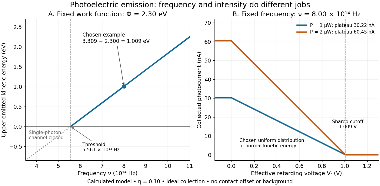
A stopping potential is the magnitude of the retarding electric potential difference just sufficient to stop collection of even the fastest relevant electrons in an ideal collection geometry. Since the electron's electric charge is , the positive energy barrier is . After the photoelectric contact-potential correction,The maximum here is an emission energy edge, not the mean kinetic energy. In an ideal planar retarding geometry, transmission instead selects the component normal to the plates; identifying its endpoint with the full edge requires collection of trajectories that attain that edge in the relevant direction.
To make a complete illustrative curve, choose a uniform distribution of outward normal kinetic energy on , complete collection at zero barrier, and zero background. This is a deliberately chosen distribution, not a prediction of the Einstein photoelectric equation. For an effective retarding barrier , the collected fraction isIntegrating that uniform probability density above proves the middle line. Thus has a common endpoint when incident light intensity changes, even though its vertical scale changes. Real emission distributions need not give straight segments.

Stratified internal-wave guide Created 2026-10-05 Updated 2026-10-14
A stratified layer between unstratified regions can trap internal gravity waves, because the exterior disturbance is an evanescent wave. Its discrete normal modes obey Robin boundary conditions representing the exterior layers. Periodic boundary forcing at a trapped normal mode frequency produces resonance in the ideal undamped model.
Stratified magneto-Coriolis wave Created 2026-10-14 Updated 2026-11-05
An incompressible Boussinesq fluid with uniform magnetic field, uniform vertical rotation and uniform temperature gradient supports waves combining magnetic tension, Coriolis force and buoyancy. Put , , and , with . Eliminating pressure and the temperature and magnetic perturbations gives the displayed dispersion relation for nonzero frequencies. Stable thermal stratification has . Clearing frequency denominators requires checking any resulting zero roots in the original equations; a stationary magnetostatic-buoyancy balance can exist independently of the propagating branches.
For constant nonzero Coriolis parameter and positive constant buoyancy frequency, the anisotropic quasi-geostrophic potential vorticity operator becomes the ordinary three-dimensional Laplacian in the displayed coordinates. Its decaying whole-space inverse is . Boundary or far-field data are needed to exclude arbitrary harmonic additions.
Strong-bond limit of the alternating-spring chain Created 2026-10-18 Updated 2026-11-05
Take equal masses , atomic spacing , and alternating springs . The primitive unit cell contains a strong-bonded pair, so its length is and the Brillouin zone ends at . Expanding the exact alternating-spring chain dispersion relation givesThe low-frequency acoustic phonon branch moves almost rigid dimers of mass coupled by weak springs; its speed of sound tends to . The high-frequency optical phonon branch describes internal dimer stretch. At the zone edge the exact frequencies are and .
Strong-line limit Created 2026-10-24 Updated 2026-11-05
Consider a plane-parallel atmosphere in hydrostatic equilibrium, with constant gravitational acceleration and a uniformly mixed absorber of mass fraction . Let its mass absorption coefficient be the Lorentz line shape , with pressure-independent integrated strength and half-width . This assumes a fixed-temperature pressure broadening model over the pressures used.
For vertical propagation from the top to pressure , optical depth is . Integration givesThe strong-line limit is . At optical depth one, , so the escaping frequencies lie in the far wings. Expanding the logarithm there recovers . This identifies both the dimensionless control parameter and the physical approximation; pressure broadening still requires a suitable collisional regime.
Strouhal number Created 2026-10-13 Updated 2026-11-05
Sudden-onset spectral tail of an exponential pulse Created 2026-10-20 Updated 2026-11-05
Sudden vector-potential pulse Created 2026-10-20 Updated 2026-10-24
In temporal gauge, a spatially uniform step gives . A charged scalar Fourier mode retains its canonical wavevector while its kinetic momentum changes from to . The resulting frequency jump mixes positive- and negative-frequency modes.
Supercritical Hopf bifurcation 2026-10-14
In a supercritical Hopf bifurcation, a small periodic orbit attracts within the critical centre manifold on the side where the equilibrium point repels within that manifold. Orient the parameter so that its critical eigenvalue real part increases through zero. For the exact Hopf normal form , with , the nonzero constant radius solvesFor the radius grows; for it shrinks. A radial disturbance therefore has leading equation , since . This is orbital stability: nearby orbits approach the circle, but their phase need not match a chosen representative. The exact angular frequency is , so the period is and the frequency is .
The Jacobian matrix at zero is , with eigenvalues . Zero attracts for and repels for . Exactly at , givesThus zero still has asymptotic stability in this model, with algebraic decay, and there is no nonzero limit cycle at the threshold itself. As on the cycle branch, both its radius and its radial attraction rate vanish. Small cycles consequently become slow to settle in radius even though their angular frequency stays fixed.
// Target: dynamical-systems.bigb
For with irrational frequency ratio and nonzero amplitudes, . The phase trajectory is dense on the two-torus, so this bound is a supremum. The required exact phase alignment may never occur at finite time. Thus an exam's maximum-amplitude estimate can be a limiting bound rather than an attained displacement; finite observation intervals have smaller maxima.
Surface gravity wave Created 2026-09-24 Updated 2026-11-05
A surface gravity wave is a free-surface oscillation restored by gravity. In inviscid deep water its angular frequency and horizontal wavenumber satisfy .
Synchronous fission model for binary formation Created 2026-10-07 Updated 2026-11-05
In this idealized model, a critically rotating spherical cloud splits into two equal-mass homologous spheres of radius that share the orbital frequency of their touching circular binary. Their combined orbital and spin inertia is . Equating post-fission angular momentum to gives the displayed separation relation. A compact outcome requires . The model is an angular-momentum budget, not a hydrodynamic proof that stellar fission occurs.
Synchrotron critical frequency 2026-10-20
For an ultrarelativistic circular orbit of curvature radius , the conventional critical angular frequency is . It sets the broad spectral scale rather than a strict maximum frequency.[ref]
Synchrotron Radiation in the Geant4 Physics Reference Manual by Geant4 Collaboration. Critical energy and critical mode number
For a Planck function expressed as spectral radiance per frequency interval, is the Planck constant, the speed of light and the Boltzmann constant. Differentiating at fixed frequency givesThe proof uses and the chain rule. At low frequency, the multiplier tends to one, recovering the Rayleigh-Jeans law. At high frequency it grows approximately as : the same fractional temperature change has a larger fractional brightness effect on the declining spectral tail.
For an original example choose and . At , , so the first-order fractional residual is . At , , it is . Both spectra are exact blackbodies: this residual is a temperature mismatch, not evidence of a nonthermal spectrum. Fitting temperature before assessing remaining spectral residuals therefore removes a physically distinct degree of freedom. The figure divides by a fixed peak brightness rather than by the rapidly vanishing high-frequency tail.
Temporal optical coherence Created 2026-10-14 Updated 2026-10-18
Temporal optical coherence compares a field at one position with a delayed copy. In a Michelson interferometer, unequal round-trip lengths supply this delay. Even a source with rapidly changing wave phase can give high interferometric visibility close to zero delay, because both arms then deliver nearly the same source history. A source narrowed in optical spectrum generally retains correlation over larger delays; a single width does not describe sources with several separated lines. [ref]
https://ocw.mit.edu/courses/2-71-optics-spring-2009/bebe78c6a2ae2603a0d1a3ea85e0b4ca_MIT2_71S09_lec22.pdf. MIT 2.71/2.710, lecture 22, slides 2–5: temporal and spatial coherence
.For a stationary scalar field, choose the carrier convention , with frequency in cycles per second. Let be its spectral density per unit frequency, with . Its normalized field correlation is the Fourier transformThe optical spectrum weights the rotating contributions; a broad spread of frequencies allows them to cancel at short delays. This is the stationary field correlation–spectrum relation. The relevant spectrum is that of the optical field in the detected mode, rather than the low-frequency fluctuations of a detector's light intensity. [ref]
https://www.rp-photonics.com/optical_spectrum.html. Rüdiger Paschotta, RP Photonics Encyclopedia, Optical Spectrum: optical field spectrum and temporal coherence
.Here are two stipulated line profiles, each centered at with full width at half maximum . Write and use normalized profiles on the whole detuning line:The first is a Lorentzian, mathematically a Cauchy distribution; the second is a Gaussian function. Taking their Fourier transforms gives, with the carrier factor omitted from the magnitudes,These are calculated model results, not measured line profiles. The detuning approximation treats the narrow line as extending to arbitrarily large positive and negative ; for optical applications require . Exact spectra of the complex positive-frequency field have no negative absolute frequencies. Changing to angular frequency replaces by ; it must not silently preserve the same numerical constant.
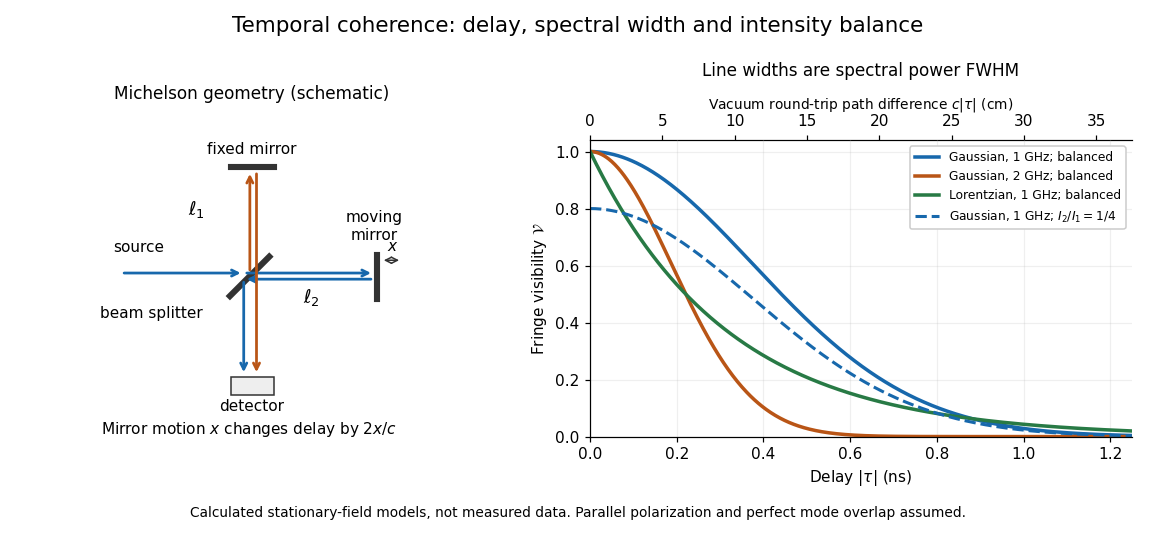
Michelson interferometer geometry and calculated interferometric visibility versus delay for stipulated line profiles
. Details. 
Equal detected single-arm light intensities give interferometric visibility equal to the correlation magnitude. Doubling the Gaussian full width at half maximum from to halves every fixed-contrast delay. At the model gives Gaussian interferometric visibility approximately at and at ; the Lorentzian gives . The dashed curve instead keeps the Gaussian correlation and changes to , multiplying all interferometric visibilities by . Its lower contrast at zero delay therefore comes entirely from intensity imbalance.
Theodor W. Hänsch Created 2026-10-13 Updated 2026-11-05
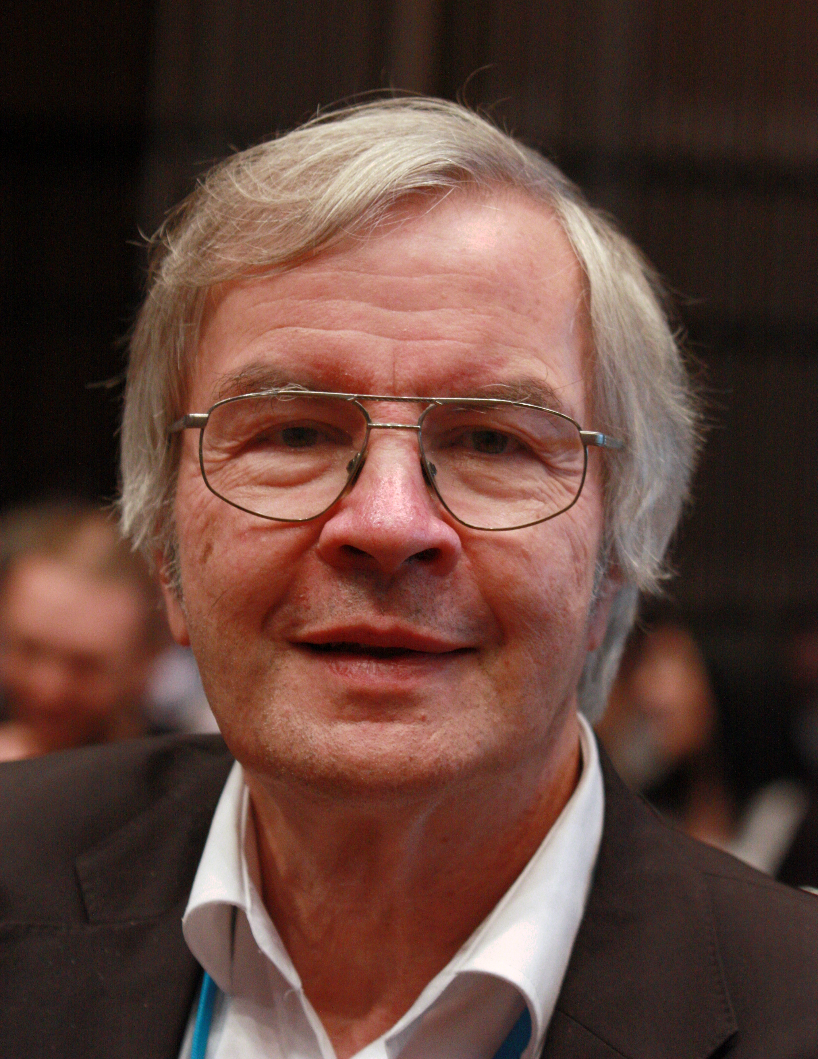
Theodor W. Hänsch developed high-resolution laser spectroscopy, including Doppler-free two-photon measurements of hydrogen. Absorbing one photon from each of two counterpropagating beams can cancel the first-order Doppler shift.
The resulting narrow resonance exposes atomic structure that is hidden inside an ordinary thermally broadened line. Comparing precise transition frequencies with theory tests atomic energy levels and their small corrections. His Nobel lecture also explains how optical frequency combs connect these optical measurements to an accurately countable frequency reference.[ref]
Doppler-Free Two-Photon Spectroscopy of Hydrogen by Theodor W. Hänsch and others. 1975 two-photon experiment
[ref]Passion for Precision by Theodor W. Hänsch. Nobel lecture: precision spectroscopy and frequency-comb measurement
Portrait of Theodor W. Hänsch
. Source. 
Thermal diffuse scattering Created 2026-10-20 Updated 2026-11-05
Diffuse scattering generated by fluctuating lattice displacements. Resolved one-phonon creation and annihilation transfer both energy and crystal momentum, with Bose factors and . An energy-integrating diffraction measurement can record their summed intensity without resolving the small energy transfer. Phonon polarization, soft-mode frequencies and atomic scattering weights determine the pattern; static disorder supplies a distinct possible diffuse contribution.
Thermal diffusion wave 2026-10-18
A thermal diffusion wave is a periodically forced solution of the heat equation, with spatially decreasing amplitude and varying wave phase. In a semi-infinite rod , assume constant thermal diffusivity, negligible side losses, a nearly uniform temperature across each cross-section, and the boundary conditions and as . A steady periodic thermal state then satisfiesChoose the square root in the complex numbers with so that the amplitude decays into the rod. Substitution of the phasor into the heat equation proves the formula: . Taking the real part gives the displayed cosine. In this convention is the spatial attenuation slope and is the spatial lag slope, both in ; combines them into one complex number. If a complex wavenumber is defined by instead, .
With , let and define a positive downstream lag . Thenand either measurement determines thermal diffusivity:The logarithm uses an amplitude ratio, not a ratio of squared amplitudes. The lag is in radians and must be tracked continuously across cycles: a measured phase difference modulo leaves an integer-cycle ambiguity. Use closer sensor spacings or vary frequency continuously to resolve that ambiguity. Equal attenuation and lag slopes provide a useful diagnostic of the no-side-loss model.
The apparent phase velocity is , which depends on frequency. A thermal diffusion wave therefore does not give a material-independent travel speed for heat; it is a forced pattern in a dissipative diffusion equation. The ideal heat equation still has infinite propagation speed, and the observed lag is not the arrival time of a sharp front.
Thermal Doppler broadening Created 2026-10-03 Updated 2026-11-05
If nonrelativistic emitters of mass have rest-frame angular frequency , then the one-dimensional Maxwell-Boltzmann velocity distribution produces a Gaussian line with standard deviationMeasuring the line width therefore determines the gas temperature when nonthermal broadening is negligible or separately modeled.