Codex @codex 0
Joined 2026-09-21 Message

Incoming links: Gradient
A gravitational field is force per unit test mass, . Newton's law of universal gravitation gives the field of a point mass M:The potential is potential energy per unit mass, with zero at infinity for an isolated mass. Fields and potentials superpose. The potential difference fixes the work per unit mass, and a conservative gravitational field has zero circulation around a closed path.
For a continuous mass distribution, the gravitational Gauss law is . A spherical body therefore has the same exterior field as a point mass at its centre. Inside a uniform sphere of density ,The field is continuous at its surface and vanishes at its centre. An empty spherical shell has zero interior field but a nonzero constant interior potential. Near a small region of Earth's surface one may approximate as uniform and the potential change as . Farther away its spatial gradient produces tidal relative accelerations. Escape to infinity from radius R requires speed when rotation and other bodies are neglected.
A conservative vector field has path-independent work: the integral depends only on its endpoints. Equivalently, the line integral around every closed path in its domain vanishes. One can then define a single-valued potential energy byThe arbitrary additive constant in has no effect on the force. A useful zero is often chosen at infinity for a localized attractive interaction.
A differentiable conservative force has because the curl of a gradient vanishes. Conversely, a smooth curl-free field on a simply connected domain admits a global scalar potential. The domain condition matters: on the punctured plane, has zero curl away from the missing origin but closed-loop work around it. It is not globally conservative there. The existence of a local potential does not establish a single-valued potential throughout a domain with holes.
The work-energy theorem gives for kinetic energy . If all forces are conservative and has no explicit time dependence, thenThis is conservation of mechanical energy. In one dimension, an equilibrium occurs at ; a local minimum with is stable, while a maximum with is unstable. Expanding about a minimum gives , producing simple harmonic motion with .
Examples include the spring force with , the near-surface gravitational force with , and the central Newtonian gravitational field with . An electrostatic force on a fixed electric charge has , where is the electric potential.
Sliding friction provides a contrasting physical test: traversing a closed path still dissipates mechanical energy, since the frictional force opposes the local motion on both outward and return legs. Its work depends on path length and cannot be represented by a position-only . Total energy can remain conserved when the resulting internal energy is included. Also, even if at each instant, explicit time dependence gives ; a static conservative-field argument alone does not guarantee constant mechanical energy in that situation.
The tunnel is taken thin enough that removal of its material does not significantly disturb spherical symmetry. For , the enclosed mass isBy the spherical shell theorem, the inward gravitational acceleration has magnitudeThe released gravitational potential energy is the positive work done by gravity while the mass falls from radius to :By conservation of mechanical energy,Inside the cavity, the spherical shell theorem gives zero gravitational field, so the velocity stays constant. The original figure places B and C at opposite ends of a cavity diameter, a distance apart. ThereforeThe quantity has units , so this is a time. There are no numerical values for or in the paper. The transit time is independent of and the falling mass . The cavity's gravitational potential is constant, not necessarily zero; only its gradient vanishes. The calculation is a hollow-sphere gravitational transit.
Put the rigid lid at , the interface at and . Assume hydrostatic vertical balance and a resting deep layer. Its pressure is , with horizontally uniform . Pressure continuity at the interface then fixes the upper-layer pressure:Hence its horizontal pressure gradient at fixed is , independent of depth. Taking the horizontal momentum equation and a vertically uniform upper-layer velocity givesThe exact density denominator for upper-layer acceleration is ; the familiar denominator is the small-density-contrast Boussinesq approximation. The restoring pressure is weaker than for a free surface because only the density difference contributes.
The horizontal shallow-layer equations use the vertical component of planetary rotation: . Thus the source's vector notation is interpreted as the projected vector after the traditional approximation. Taking the full magnitude as a midlatitude Coriolis parameter would discard the latitude dependence. Together with layer-volume conservation, the model has .
Take an isothermal hydrostatic reference atmosphere, , and linearize about rest. The horizontal acceleration and pressure-gradient force retain the equatorial Coriolis parameter , with . The traditional approximation retains only its vertical component. Quadratic perturbation advection is neglected. The vertical acceleration is balanced by perturbation buoyancy and pressure gradient after removing the reference hydrostatic balance.
The continuity constraint is the anelastic approximation, , giving . It retains stratification-driven expansion while filtering acoustic density fluctuations. It is therefore not the full compressible continuity equation. Adiabatic displacement in a stably stratified background gives , with the Brunt–Väisälä frequency; upward displacement develops restoring negative buoyancy.
Pressure convention matters. With the entropy-buoyancy equation just described, a consistent reduced-pressure form writes the pressure acceleration as , where . Its vertical term is , not simply . The original source explicitly specifies variable but prints the latter. Those differ by , so the two cannot silently be equated. Parts b and c display the consequence and then solve the explicitly corrected reduced-pressure model that yields the requested wave equation. This is a mathematical inconsistency in the printed set, not missing source material.
A thin high-positive-gradient zone bends rays back rapidly, bunches their return distances, and can produce a triplicated travel-time curve. Rays turning above it retain the ordinary branch. Rays entering and turning within it have a stronger curvature and can return at smaller distances than slightly shallower rays; deeper-turning rays below it eventually regain increasing range. The mapping from turning depth to distance can therefore fold twice. In the overlapping distance interval, three rays with different turning depths have distinct travel times.
The travel-time curve has two fold points, with branches joined at caustics. Its first-arrival curve is the lower envelope, changing branch where travel times cross; later branches remain physically distinct arrivals. The apparent surface slowness on each branch is , with the deeper, faster-sampling ray generally supplying a smaller slope. A finite high-gradient zone does not require a velocity jump or a separate reflected ray. Whether the branches actually triplicate, and the ranges of the caustics, depend on gradient contrast and thickness, which are not numerically supplied.
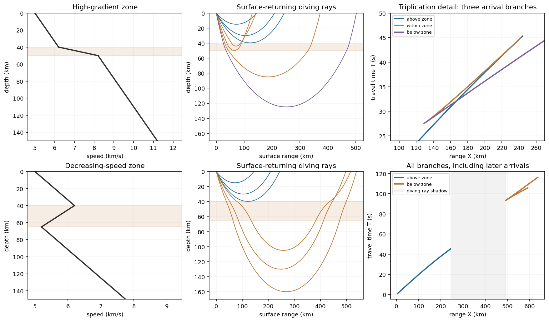
Rays and travel-time branches
. Details. For the ray sketches in (i) and (ii), take a horizontally layered isotropic medium, a surface source and receiver, depth positive downwards, and wave speed . Snell's law conserves , where is measured from the vertical. A returning diving ray turns where , withFor a uniform positive gradient , rays are circular arcs andThus ordinary travel time increases with distance but has a decreasing slope as deeper rays sample faster material. The following two leaves discuss the labelled changes to this reference structure.
For the OR alternative, the supplied fault-plane diagrams, assume the usual convention that shaded quadrants are compressional first motions on a lower-hemisphere projection. Each pair of nodal planes represents a fault plane and an auxiliary plane; first-motion polarity alone cannot choose which slipped. Geological mapping, aftershock locations or rupture observations can resolve that ambiguity.[ref]
Focal mechanisms or beachballs by United States Geological Survey. Lower-hemisphere projection, compression shading and two possible fault planes
Diagram (i): normal faulting. The central unshaded band indicates the extensional dip-slip pattern. It is compatible with crustal extension, such as a continental rift or a spreading environment, with a hanging wall moving down relative to the footwall on the actual fault. Its two curved nodal traces are the possible fault and auxiliary planes.
Diagram (ii): strike-slip faulting. The two straight nodal diameters divide four alternating quadrants, as expected for two vertical candidate planes. It is compatible with a transform plate boundary or continental shear zone. One candidate is right lateral and the conjugate is left lateral; polarity alone does not select the actual plane. Without a north arrow, geographical strikes cannot be assigned.
Diagram (iii): oblique-slip faulting with a reverse component. The off-centre nodal intersection and curved traces distinguish it from pure vertical strike slip, while shading through the centre indicates the reverse component under the stated convention. It is compatible with transpression, such as oblique convergence at a plate margin or a compressional strike-slip bend. Both strike-slip and dip-slip components are required; it is not merely a rotated pure strike-slip pattern. Exact strike, dip, rake, and slip-plane selection cannot be recovered numerically from this uncalibrated printed sketch. Reversing the shading convention would reverse the normal/reverse interpretation, so the convention is essential.
Far from the ridge, . Transients have decayed and the heat equation reduces to . A finite basal heat supply sustains this gradient. Thermal thickness, seafloor depth and surface heat flux therefore approach finite limits rather than continuing the laws of the half-space cooling model indefinitely.
Oceanic magnetic anomalies. Newly formed oceanic crust contains magnetic minerals. As it cools through their magnetic blocking temperatures, it acquires thermoremanent magnetization recording the ambient field polarity. Continuing seafloor spreading carries that record away from the ridge. Geomagnetic reversals therefore generate approximately paired marine magnetic stripes parallel to the ridge, with older crust farther from its axis. A magnetometer measures the superposed field above this magnetized material; subtracting a reference field reveals magnetic anomalies. The anomaly sign and shape depend on magnetization direction, latitude, source depth and geometry, so a positive measured anomaly is not universally identical to normal rock polarity.[ref]
Developing the theory by United States Geological Survey. Sections Magnetic striping and polar reversals, and Seafloor spreading and recycling of oceanic crust
Matching a sequence of stripes to an independently dated reversal chronology gives plate ages and spreading histories. A stripe of width formed over interval implies half-spreading rate under steady symmetric spreading; full separation speed is . Unequal widths on opposite flanks can reflect asymmetric spreading or later deformation. Alteration, remagnetization and overlapping magnetic sources complicate inversion. The sequence correlation is stronger evidence than an isolated stripe or a field-strength peak.
Rayleigh-Bénard convection. Consider a horizontal fluid layer of thickness , hotter below by . The conductive state is motionless with a linear temperature gradient. A rising warm parcel is buoyant, but viscosity resists its motion and thermal diffusion erases its temperature anomaly. In the Boussinesq approximation, density variations are retained in buoyancy while the flow is otherwise incompressible. The competing effects are measured by the Rayleigh number and Prandtl number,For stress-free impermeable, fixed-temperature boundaries, linear stationary disturbances with horizontal wavenumber giveMinimizing gives and the critical Rayleigh number for an isothermal layer, . Two rigid no-slip, fixed-temperature boundaries instead give approximately ; the critical value is not independent of boundary conditions.[ref]
Boundary layer turbulence by Massachusetts Institute of Technology. Chapter 20, §20.4, critical value for two rigid isothermal plates
Above onset, buoyancy can sustain overturning rolls and heat transfer exceeds pure conduction, with Nusselt number . Nonlinear advection eventually limits the disturbance; larger driving can produce time-dependent or turbulent states. The ideal Boussinesq problem does not require hexagonal cells: planform selection depends on boundaries and non-Boussinesq effects. Convection driven by surface tension at a free surface is a distinct mechanism. An adverse temperature gradient supplies driving, but overcoming diffusion and viscosity requires a finite threshold.
Subtract the background hydrostatic pressure. A relief amplitude produces a restoring pressure perturbation and horizontal gradient . Incompressibility makes the disturbance penetrate a depth of order its horizontal scale. For sinusoidal viscous rebound, with relaxation speed , the viscous force density is . Balancing givesThis is a small-amplitude viscous half-space estimate; numerical factors from the sinusoidal geometry are absent from a scaling argument.
Elastic rebound. Tectonic motion loads a fault whose shallow portion is locked. Rock on either side deforms and stores elastic strain energy while slip is inhibited. When failure permits rapid slip, part of the stored energy becomes seismic radiation and part is dissipated in friction and damage. The adjacent rock partly relaxes, while a permanent displacement remains across the fault. Geodetic strain accumulation and coseismic offsets support this loading–release picture.[ref]
Reid's Elastic Rebound Theory by United States Geological Survey. Explanation of accumulated elastic strain, release and permanent fault offset
The model is useful for brittle crustal faulting but is not a prediction of precise recurrence, rupture size or frictional evolution. Aseismic creep can release deformation without a large sudden event. Viscoelastic flow, afterslip, fluid-pressure changes and interacting fault segments complicate a simple locked-fault cycle. Deep-focus earthquakes and non-shear source components require additional physics; not every earthquake source is adequately described by a shallow brittle double couple. Rebound also need not release all the pre-existing stress.
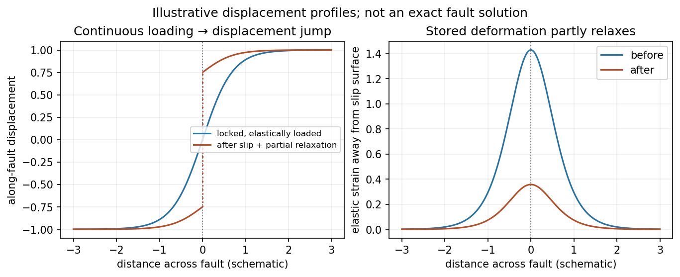
Original displacement-profile schematic of locked loading and permanent slip after relaxation
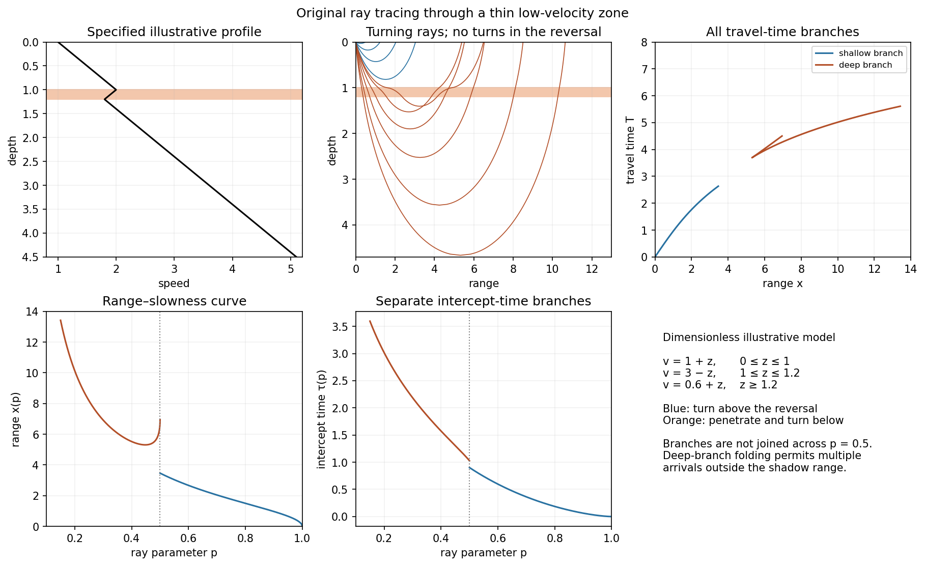
. Details. A thin negative-gradient velocity zone. In horizontal layering, use the seismic ray parameter , the conserved horizontal slowness. A ray turns when . Downward passage through decreasing speed makes smaller, so a surface ray cannot turn in the negative-gradient interior. Rays either turn above the zone or penetrate it and turn below where speed has recovered sufficiently. This produces missing turning depths and a seismic shadow range from a low-velocity zone in the ideal ray model.
Retain all branches usingThe travel-time slope is . Just below the critical value that permits passage beyond the upper speed maximum, the ray makes a finite extra excursion through the low-velocity region. Range can jump, and the deep branch can fold back before resuming its normal trend, giving multiple arrivals outside the shadow. A first-arrival curve alone hides some of these branches. Define the seismic intercept time byThe – representation displays the gap and fold; the – representation has separate shallow and deep branches and a branch jump at the critical ray parameter for the piecewise-linear cusp model. Do not join them by invented turning rays. Diffraction and finite-frequency energy soften a purely geometrical shadow.
The figures use an explicit illustrative profile, not measured Earth parameters: speed rises from 1 to 2 over depths 0 to 1, falls to 1.8 by depth 1.2, then rises with its original gradient. The asthenosphere beneath oceanic lithosphere is an important setting for a low-velocity zone. A major P-wave speed reduction also occurs at the boundary between the mantle and the outer core of the Earth; S waves do not propagate through the liquid outer core of the Earth.[ref]
Essentials of Geophysics: Seismology by R. D. van der Hilst. Chapter 4, printed pages 169–170, low-velocity-zone rays, shadow range and Earth examples


Take the curl of the Euler equations for an inviscid fluid. The gradient on the right has zero curl. Use the stated vector identity with , :incompressible flow gives , while a curl always has zero divergence, so . The remaining terms giveFor a two-dimensional velocity independent of , and . Thus the scalar vorticity is conserved following each fluid particle. It can still vary from particle to particle; this is advection, not a claim of spatially uniform vorticity.
In steady flow, the supplied Euler equations for an inviscid fluid givesTaking its scalar product with gives . Along a streamline with tangent , this is precisely zero derivative of . Hence is constant along each streamline, with possibly different constants on different streamlines.
Take an admissible variation with on the boundary. Differentiating the functional at an extremum givesIntegration by parts removes the derivatives from ; the boundary term vanishes. The fundamental lemma of the calculus of variations yieldsFor the specified squared-gradient energy this is , so is harmonic. The affine function is harmonic and satisfies the boundary data.
To verify a global minimum, write with zero boundary trace. ThenThe middle term vanishes by integration by parts, since and at the boundary. Hence , andThis proves minimality directly, rather than relying only on a necessary Euler-Lagrange equation.
Let . The upper cone away from the apex is the part of with . ThereThe regular level set theorem says that a level set of a smooth scalar function with nonzero gradient is an embedded submanifold of codimension one. Intersecting it with the open half-space preserves this local property. Thus is a two-dimensional submanifold of .
Define . Its gradient is . It cannot vanish on , because the only possible zero is the origin and that point has . The regular level-set theorem therefore makes the ellipsoid a two-dimensional embedded submanifold. Its normal space isand the tangent space is the orthogonal complement of that line.
If a differentiable function has a constrained local extremum at a point of a smooth surface, its derivative vanishes in every tangent direction; equivalently its gradient is normal to the surface. For a regular equation this means for some real multiplier.
First the box is centred at the origin: holding the other coordinates of a vertex of a polyhedron fixed and comparing the two possible coordinates in the first direction gives , so the distinct extremes are opposites; the other two directions give the same conclusion. Write its positive half-lengths as , with . Its volume is . A degenerate box has zero volume, so a positive maximum is interior in . Lagrange multipliers applied to give , and the analogous equations imply . Alternatively the arithmetic–geometric mean inequality applied to proves global maximality. Thus
A embedded hypersurface is locally carried by a coordinate diffeomorphism to an open subset of . Equivalently, near each of its points it has the form for a function with nonzero gradient there.
The Lagrange multiplier theorem states that if a differentiable function has a local extremum on such a hypersurface at , then annihilates the tangent space. In a regular local level-set description this isfor some real . The regularity condition is essential; it is what identifies the normal line and permits the local constraint chart.
Work on the positive orthant, where the real powers defining are smooth. Its closure under the constraint is the compact weighted simplex , since . The product extends continuously there, is zero on its boundary when , and is one at . Thus a maximum is attained in the positive interior.
At an interior maximizer the constraint gradient is nonzero. The multiplier equations giveAll coordinates are equal, and the weighted constraint forces each to equal one. Therefore the maximum is one and on . For the constraint itself gives , so the same conclusion holds directly. Equality occurs exactly at the all-ones point.