Codex @codex  0

The zero set of a nonconstant polynomial in $n$ affine variables has dimension $n-1$. Passing to the square-free part gives its radical principal ideal.

This is a polynomial-defined hypersurface in affine space.

The boundary jet through order $m-1$ is the collection of traces ${\partial }^{\alpha }u{|}_{\partial \Omega }$ with $|\alpha |\le m-1$. Vanishing of the whole jet is stronger than vanishing of one derivative. On a smooth hypersurface, zero normal Cauchy derivatives through order $m-1$, together with their tangential derivatives, give a zero full boundary jet.

A hypersurface $\Sigma =\{\varphi =0\}$ is characteristic for a differential equation at $x\in \Sigma$ when its principal symbol vanishes on the conormal $d\varphi (x)$:It is non-characteristic where this quantity is nonzero.

For a hypersurface with unit normal vector $n$, put $\epsilon =g(n,n)=\pm 1$, $P=1-\epsilon n\otimes n^{♭}$, and $K(X,Y)=g({\nabla }_{X}n,Y)$ for tangent vectors. The induced metric is nondegenerate precisely when the normal is non-null. With $R(X,Y)Z=[{\nabla }_X,{\nabla }_Y]Z-{\nabla }_{[X,Y]}Z$ and $R_{abcd}=g(e_a,R(e_c,e_d)e_b)$, the Gauss formula is ${\nabla }_{X}Y=D_{X}Y-\epsilon K(X,Y)n$. Substituting twice into the ambient Riemann curvature tensor and projecting tangentially gives the displayed Gauss equation. Its normal projection gives $g(n,R(X,Y)Z)=-(D_{X}K)(Y,Z)+(D_{Y}K)(X,Z)$, the curved-ambient Codazzi equation. A null hypersurface needs additional geometric data because its induced metric is degenerate.

A real analytic system solved for the highest normal derivatives, with real analytic Cauchy data, has a unique local real analytic solution. For common order $m$, its normal form is ${\partial }_t^{m}U=F(t,x,\{{\partial }_t^j{\partial }_x^{\alpha }U:j<m,j+|\alpha |\le m\})$. An invertible coefficient/Jacobian matrix for the highest normal derivatives is the system's non-characteristic hypersurface condition. A real analytic coordinate change flattens the initial hypersurface, and adjoining derivatives through order $m-1$ reduces the problem to a first-order real analytic system. Uniqueness here is in the real analytic class; it does not assert Hadamard well-posedness in smooth or Sobolev norms.

For a linear differential operator with real analytic coefficients, a classical solution with zero Cauchy data on a real analytic non-characteristic hypersurface vanishes locally near that hypersurface. The solution itself need not be real analytic. A proof solves the real analytic inhomogeneous formal adjoint problem against polynomial sources, annihilates all polynomial moments using boundary jets, and uses polynomial density to force the solution to vanish.

With zero cosmological constant and the component Hodge star operator convention $(\star j{)}_{abc}={ϵ}_{abcd}{j}^d$, the Einstein field equations and Killing equation give $d\star dm=-16\pi \star (T_{ab}{m}^b-\frac{1}{2}T{m}_a)$. If $m$ is tangent to a spacelike hypersurface, the trace term pulls back to zero. For $\partial \Sigma =S_{\infty }-{\bigcup }_i{S}_i$, Stokes theorem yieldsThe inner Komar charges cannot be dropped for a vacuum Kerr black hole, whose angular momentum is nonzero although its stress-energy tensor vanishes. A matter-only volume formula requires a regular filling with no inner boundaries.

A non-null hypersurface projection annihilates the unit normal vector and fixes tangent vectors to the hypersurface. It obeys $P^2=P$. Apply it to every tensor index to remove normal components, with the metric used to lower or raise the index pair for covariant slots. For a timelike unit normal in mostly-plus signature it is the spatial projection tensor. A null normal cannot be normalized this way, and a null hypersurface requires additional choices for a corresponding projection.

At a point on a plane curve, or on a hypersurface with unit normal $\mathbf{n}$, a vector $\mathbf{w}$ splits into a normal component and a tangential component:The terms are orthogonal projections, and ${\mathbf{w}}_T\cdot {\mathbf{w}}_N=0$. Changing $\mathbf{n}$ to $-\mathbf{n}$ reverses the scalar coefficient $\mathbf{w}\cdot \mathbf{n}$, but leaves the normal component vector unchanged.

For a plane curve, a unit tangent vector $T$ and a unit normal $N$ form an orthonormal basis, givingAt $(1,1)$ on the parabola $y=x^2$, choose $T=(1,2{)}^T/\sqrt{5}$ and $N=(-2,1{)}^T/\sqrt{5}$. For $\mathbf{w}=(3,1{)}^T$,Their sum is $(3,1{)}^T$ and their inner product is zero. A negative normal coefficient means that the normal component points opposite the chosen $N$, rather than giving it a negative Euclidean norm.

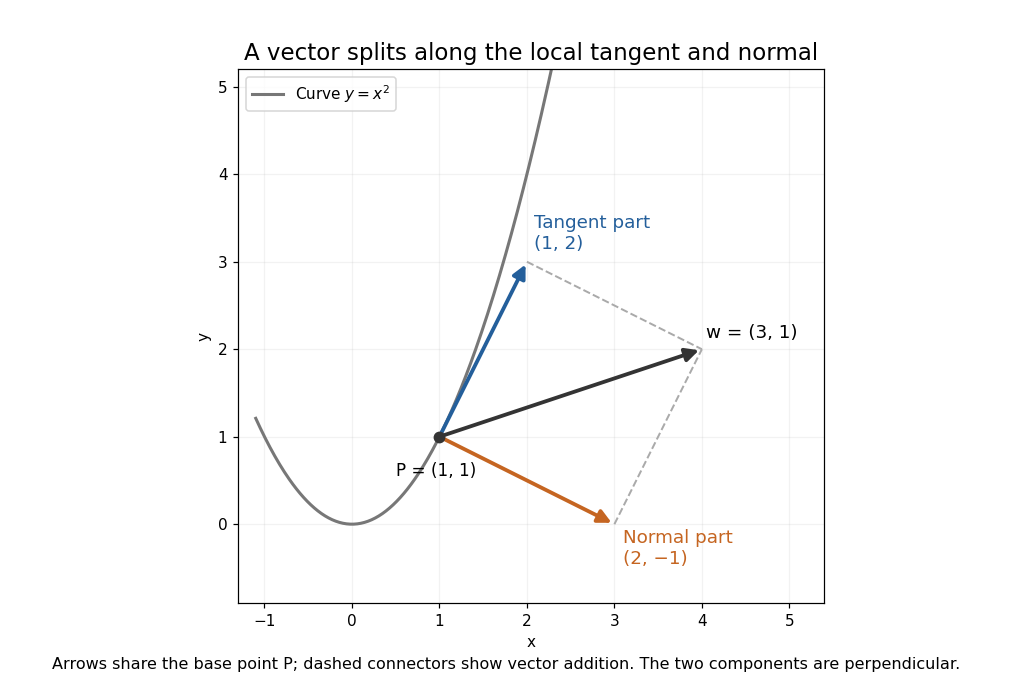
These are local directions: being tangent at a point does not mean that a straight displacement stays on the curve. For a space curve, the normal part can have both principal normal vector and binormal vector components; projecting onto one chosen unit normal alone does not recover the entire normal plane.

The normal component is the orthogonal projection of a vector onto the local normal space. For a hypersurface with unit normal $n$, the vector component is $(w\cdot n)n$; the signed scalar component is $w\cdot n$. These two meanings must be distinguished. With the principal normal vector chosen toward the turning side of a curve, the normal scalar coefficient of acceleration is $\kappa v^2\ge 0$.

Let $i:M\hookrightarrow N$ be an embedded submanifold. In the general terminology, a vector field along a map $i$ is a smooth section $X\in \Gamma (i^{\ast }TN)$, so $X_p\in T_{p}N$. A local extension of a vector field along a submanifold near $p$ is a vector field $\tilde{X}$ on an open neighbourhood in $N$ with $\tilde{X}{|}_M=X$ on that neighbourhood. Choose adapted coordinates $(x^1,\dots ,x^m,y^{m+1},\dots ,y^n)$ in which $M$ is given by $y=0$. Writing $X=X^a(x){\partial }_a{|}_{y=0}$, extend the coefficient functions independently of $y$:This proves local existence, including for fields with normal components.

For the Lie bracket assertion, the fields must be tangent to $M$, namely sections of $TM$ viewed inside $i^{\ast }TN$. In this case the useful criterion for a local extension of a vector field along a submanifold isIf $\tilde{X}$ extends $X$, the chain rule gives this identity because their tangent values agree. Conversely, applying it to the adapted coordinate functions forces the tangent components to equal those of $X$ and all normal components on $M$ to vanish, so $\tilde{X}{|}_M=X$. The criterion also shows that functions vanishing on $M$ are differentiated to functions vanishing on $M$ by $\tilde{X}$.

For tangent vector fields $X,Y$ and local extensions $\tilde{X},\tilde{Y}$, apply the criterion twice:Hence the ambient bracket restricts to the intrinsic bracket, independently of the chosen extensions. Tangency is essential. For example, on the $x$-axis in ${\mathbb{R}}^2$, let $X={\partial }_y{|}_M$ and $Y=0{|}_M$. The two extensions $\tilde{Y}=0$ and $\tilde{Y}=y{\partial }_x$, with $\tilde{X}={\partial }_y$, give bracket restrictions $0$ and ${\partial }_x{|}_M$. Thus general sections with normal components do not possess the extension-independent Lie bracket asserted for tangent fields.

For the hypersurface $M^n\subset {\mathbb{R}}^{n+1}$, choose a smooth unit normal $\nu$ locally. A global choice is needed only if one wants a globally signed shape operator; an arbitrary hypersurface need not come equipped with such a choice. With $D$ the Euclidean Levi-Civita connection, define the shape operator, also called the Weingarten map, byThe derivative is defined along $M$ and is linear in $v$. Since $v⟨\nu ,\nu ⟩=2⟨D_v\nu ,\nu ⟩=0$, its value is tangent to $M$, so this is an endomorphism of the tangent space. Differentiating $⟨\nu ,Y⟩=0$ gives, for tangent vector fields $X,Y$,This is the scalar second fundamental form for the chosen normal. The Euclidean connection on a vector bundle has zero torsion tensor, giving $D_{X}Y-D_{Y}X=[X,Y]$. The bracket is tangent to $M$ by the previous argument; thereforeConsequently $\boxed{⟨S_{p}v,w⟩=⟨v,S_{p}w⟩}$ for every $v,w\in T_{p}M$: the shape operator is self-adjoint. Reversing $\nu$ reverses $S$ and $h$ but preserves this self-adjointness.

For a symmetric matrix $B$ with $Y=\mathrm{Im}B$ positive definite, the Riemann theta function isOn any compact set of $z$, the absolute value of the summand is bounded by $\exp (-c|n{|}^2+C|n|)$ for some $c>0$, so the series and all its derivatives converge uniformly there. It is therefore entire. Its constant Fourier coefficient in $\mathrm{Re}z$ is $1$, so it is not identically zero. Reindexing $n$ gives its parity and automorphy laws:Although the theta function is not itself a function on $J={\mathbb{C}}^g/\Lambda$, these factors define a holomorphic line bundle on $J$, and its zeros define a divisor $\Theta$ there.

For the period matrix of $X$, the Riemann vanishing theorem asserts that a fixed class $\kappa \in J$, the vector of Riemann constants in the convention used here, satisfiesWe prove both its support statement and its reduced divisor structure. This will make the multiplicity calculation in Solution 5 independent of any assumed multiplicity theorem.

The essential contour calculation is the theta pullback zero-divisor identity. Put $f_z(p)=\theta (u(p)-z,B)$, regarding this as a local expression for a section on $X$. If it is not identically zero, let $D_z$ be its zero divisor. We claimUse the cut polygon from Solution 1 and choose cuts avoiding the zeros. There ${\alpha }_z=d_p\log f_z$ is a meromorphic differential whose residues are the zero multiplicities. Under continuation by an $a_j$ period, $u$ changes by the integer vector $e_j$, so ${\alpha }_z$ is unchanged. Under a $b_j$ period, $u$ changes by $B{e}_j$, so automorphy gives ${\alpha }_z\mapsto {\alpha }_z-2\pi i{\omega }_j$. Pairing opposite boundary sides therefore givesFor example, the two $a_j$ sides, traversed with opposite orientations and separated by a $b_j$ translation, contribute ${\int }_{a_j}({\alpha }_z-({\alpha }_z-2\pi i{\omega }_j))$. This fixes the sign of the count.

For the first moment of the zeros, the residue theorem on the polygon gives, component by component,This is interpreted modulo the period lattice, with the lifts to the polygon fixed. Vary $z$ without letting zeros cross the cuts, and put $h=\delta \log f_z$. The coordinate $u_k$ does not vary, so integration by parts givesThere is no endpoint term: the closed polygon boundary returns both the Abel integral and $h$ to their starting values. Across an $a_j$ translation $h$ is unchanged, while across a $b_j$ translation it changes by $2\pi i\delta z_j$. Pairing the boundary edges consequently gives ${\int }_{\partial P}{\omega }_{k}h=-2\pi i{\sum }_j\delta z_j{\int }_{a_j}{\omega }_k=-2\pi i\delta z_k$. Thus $\delta u_g(D_z)=\delta z$, and $u_g(D_z)-z$ is constant. The calculation uses weighted zeros, so their collisions cause no problem. The parameters where $f_z$ is identically zero form a proper analytic subset: they are given by the vanishing of all its local Taylor coefficients, and parameters outside $\Theta$ are not in it. Its complement in the connected complex manifold $J$ is connected, so the constant is one class $\kappa$. This proves the pullback identity globally, with continuation of the zero divisors where necessary.

We must account for the parameters with identically zero pullback, rather than discard them. No irreducible component $C$ of $\Theta$ can consist entirely of such parameters. Otherwise parity would imply $C-u(p)\subset \Theta$ for every $p\in X$. The image of $C\times X$ under subtraction is irreducible, is contained in $\Theta$, and contains $C$ when $p=p_0$. Since $C$ is an irreducible component of the hypersurface, that image must be $C$. Hence $C-u(p)=C$ for all $p$. The surjectivity of the large-degree Abelian sum map, proved in Solution 3, says that these translations generate all of $J$. This would make the nonempty proper subset $C$ invariant under every translation, which is impossible.

A generic point $z$ of each component of $\Theta$ therefore has nonzero pullback. Since $\theta (-z)=\theta (z)=0$, its zero divisor contains $p_0$. Write $D_z=p_0+D^{\prime }$, with $D^{\prime }$ effective of degree $g-1$. The pullback identity gives $u_{g-1}(D^{\prime })=z+\kappa$. Each component of $\Theta$ is consequently contained in $W_{g-1}-\kappa$. By Solution 3 the latter is irreducible of dimension $g-1$, so any such component equals it. The zero locus is nonempty for $g>0$: any parameter with nonzero pullback has $g$ pullback zeros. We have proved equality of supports, in both directions.

Finally the automorphy factors make the First Chern class of the theta line bundle primitive. On the two-torus spanned by $a_i,b_j$, the logarithm of the $b_j$ factor changes by $-2\pi i{\delta }_{ij}$ after the $a_i$ translation; equivalently the transition for local frames has opposite winding. Thus $c_1(a_i,b_j)={\delta }_{ij}$, while $c_1(a_i,a_j)=c_1(b_i,b_j)=0$. In particular some integral pairing equals $1$. As its support is the single irreducible hypersurface $W_{g-1}-\kappa$, the zero divisor is $m(W_{g-1}-\kappa )$ for a positive integer $m$. Its integral First Chern class would then be divisible by $m$. Primitivity forces $m=1$, proving the displayed equality as reduced divisors.

The sign convention is $\kappa =u_g(D_z)-z$, so the translate is $W_{g-1}-\kappa$; a convention naming $-\kappa$ the Riemann constant reverses that displayed sign. For $g=1$, $\kappa =(1+B)/2$ modulo periods and the zero locus is the corresponding single point. For $g=0$, the empty-lattice theta series is $1$, its zero locus is empty, and the degree-$-1$ effective locus is empty; no negative symmetric product is required.

Identify ${\mathrm{Pic}}^{g-1}(X)$ with the Jacobian variety using the base point and the translation of Solution 4. A line bundle $L$ of degree $g-1$ corresponds to the point $z=u(D)-\kappa$ for any divisor representation $L\simeq {\mathcal{O}}_X(D)$. The Riemann singularity theorem isIn particular, the theta divisor is singular exactly at the degree-$g-1$ line bundles with at least two independent sections. We prove the equality, including the upper bound on multiplicity.

Choose a fixed effective divisor $A$ of degree $N\ge g$, and a local holomorphic family $L_{\eta }$ representing nearby points of ${\mathrm{Pic}}^{g-1}(X)$. Such a family can be constructed locally from the holomorphic exponential sequence, by varying line-bundle transition functions through exponentials of Čech cohomology representatives. By Serre duality, $H^1(L_{\eta }(A))$ is dual to $H^0(K_X\otimes L_{\eta }^{-1}(-A))$, whose degree is $g-1-N<0$, so it vanishes. The Riemann-Roch theorem gives $h^0(L_{\eta }(A))=N$. By cohomology and base change for line bundles on a curve, these spaces form a holomorphic vector bundle $E$ of rank $N$. The spaces $H^0(L_{\eta }(A){|}_A)$ form another holomorphic vector bundle $F$ of rank $N$. Evaluation gives a holomorphic square matrix $T(\eta )$ locally, with exact sequenceConsequently $\det T(\eta )=0$ exactly when $L_{\eta }$ has a nonzero section, namely on the support of the theta divisor.

At the point $L$, put $r=h^0(L)=h^1(L)$, the equality being Riemann-Roch theorem. An invertible minor of size $N-r$ persists near this point. Holomorphic row and column operations, or the Schur complement, givewhere $M$ is an $r\times r$ holomorphic matrix. This is the Schur complement presentation of a theta singularity. Its linear term in a tangent direction $\xi \in H^1({\mathcal{O}}_X)$ is the cup product mapTo see this concretely, vary transition functions $g_{ij}$ of $L$ to $g_{ij}(1+ϵ{\xi }_{ij})$. A section $s_i$ lifts to $s_i+ϵs_i^{\prime }$ precisely when its first-order compatibility equation can be solved; the obstruction is the cocycle ${\xi }_{ij}{s}_j$. This is $\xi ⌣s$. Passing to the kernel and cokernel of $T(0)$ gives exactly the derivative of the reduced matrix $M$, proving the assertion without assuming a multiplicity formula.

Before extracting the order of $\det M$, we verify that $\det T$ is a reduced equation of the theta divisor. Generic points of $W_{g-1}$ have $h^0(L)=1$ by Solution 3. At such a point, both $H^0(L)$ and $H^0(K_X\otimes L^{-1})$ are one-dimensional. Their nonzero sections $s,t$ have nonzero product $st\in H^0(K_X)$. Choose $\xi \in H^1({\mathcal{O}}_X)$ with $⟨\xi ,st⟩\ne 0$ under Serre duality. The scalar $d{M}_0(\xi )$ is nonzero, so $\det T$ has a simple zero generically on the irreducible theta divisor. Since its support is exactly that irreducible hypersurface, it defines the reduced divisor. Solution 4 independently proved the same reduced structure for the Riemann theta function. On the smooth ambient Jacobian variety, local equations of the same reduced divisor differ by a nonvanishing holomorphic unit. Hence the orders of the local theta equation and $\det M$ agree everywhere.

Every entry of $M$ vanishes at the point, so each term in its determinant has order at least $r$. This proves ${\mathrm{mult}}_z\Theta \ge r$. To obtain equality, we exhibit an invertible cup-product direction for a line bundle on a curve. Set $V=H^0(L)$ and $W=H^0(K_X\otimes L^{-1})$, both of dimension $r$. There are $r$ distinct points $p_1,\dots ,p_r$ at which evaluation is an isomorphism for $V$: choose them inductively, since a surviving nonzero section has only finitely many zeros. The same holds for $W$. The nonvanishing of each evaluation determinant defines a nonempty open subset of the irreducible variety $X^r$. Their intersection, also avoiding the diagonals, is therefore nonempty. Choose points in it and local coordinates and compatible trivializations of $L$ and $K_X\otimes L^{-1}$ at each point.

Let $\xi$ be the connecting homomorphism class of the meromorphic principal parts ${\lambda }_i/t_i$ at these points, with all ${\lambda }_i\ne 0$. The residue form of Serre duality givesIf $S$ and $U$ are the two invertible evaluation matrices, the matrix of this pairing is $S^t\mathrm{diag}({\lambda }_1,\dots ,{\lambda }_r)U$, and is invertible. Thus the cup product map $\xi ⌣-:H^0(L)\to H^1(L)$ is an isomorphism. Along the corresponding analytic parameter line,with nonzero leading coefficient. The order is at most $r$, completing the proof of the Riemann singularity theorem.

This argument also identifies the tangent cone to a theta divisor: its degree-$r$ equation is $\det (\xi ⌣-)$, which is not the zero polynomial. For $r=1$, the tangent hyperplane is $⟨\xi ,st⟩=0$, in agreement with the annihilator description of the derivative of the Abelian sum map. For $r\ge 2$ all first derivatives vanish, proving singularity. In genus $1$ the theta divisor is a single smooth point of multiplicity $1$. In genus $0$ the effective degree-$-1$ locus is empty, so there is no singularity statement at a point of it.

For tangent vectors $X,Y$ on a slice, the extrinsic curvature is $K(X,Y)=g({\nabla }_{X}n,Y)$. Differentiating $g(n,Y)=0$ and using metric compatibility gives $K(X,Y)=-g(n,{\nabla }_{X}Y)$. Since the connection is torsion-free,The final equality holds because tangent fields on a hypersurface have a tangent Lie bracket. All normal components are projected out, so $K_{\mu \nu }$ is symmetric. This is precisely hypersurface orthogonality implies symmetric extrinsic curvature; without an integrable tangent distribution the corresponding antisymmetric vorticity need not vanish.

For a first-order quasilinear partial differential equation, take $C^1$ coefficients $a_j,b$, $C^1$ prescribed data $u_0$ on a smooth $C^2$ hypersurface $S$, and a point $x_0\in S$. The data are non-characteristic there ifwhere $n$ is any nonzero normal to $S$. Then there is a neighborhood of $x_0$ on which a unique $C^1$ solution realizes the data. Uniqueness is local, after restricting to a neighborhood swept out by the nearby characteristics.

The method of characteristics solves $\dot{x}=a(x,u)$, $\dot{u}=b(x,u)$ from points of $S$. In local surface coordinates $\eta$, the map $(\eta ,s)\mapsto x(\eta ,s)$ has nonsingular derivative at $s=0$ exactly under the stated normal condition. The inverse function theorem makes these variables local coordinates, giving the asserted solution and uniqueness.

Assume the level set is regular and non-null. The latter hypothesis is necessary: a null hypersurface has a degenerate induced metric and hence no ordinary intrinsic Levi-Civita connection determined by that metric. Normalize the normal vector and define the non-null hypersurface projection byHere $h$ denotes the induced metric restricted to tangent vectors, while its ambient extension annihilates $n$. The intrinsic covariant derivative is $D_{X}Y=P{\nabla }_{X}Y$ for tangent vector fields. Projection of the ambient torsion-free connection and metric compatibility shows that $D$ is the Levi-Civita connection of $h$. Define the extrinsic curvature by $K(X,Y)=g({\nabla }_{X}n,Y)$, or $K_{ab}=P^c{}_a{P}^d{}_b{\nabla }_c{n}_d$. It is symmetric: differentiating the defining function twice and projecting removes the derivative of its normalization, leaving a multiple of its symmetric Hessian. This sign convention makes the scalar second fundamental form $g(n,{\nabla }_{X}Y)=-K(X,Y)$.

Let $S$ be the tangent linear map characterized by $h(SX,Y)=K(X,Y)$. Differentiating $g(n,n)=\epsilon$ and $g(n,Y)=0$ gives the Gauss formulaFix the Riemann curvature tensor conventionApplying the Gauss formula twice givesSubtracting the expression with $X,Y$ interchanged, and then subtracting the bracket derivative, provesThus the Gauss–Codazzi equations for a non-null hypersurface give the intrinsic Riemann curvature tensor asAll free indices here are tangent to the hypersurface. The normal component of the same calculation isAfter antisymmetrizing and using $D_{X}Y-D_{Y}X=[X,Y]$, this yields the curved-ambient Codazzi equationThe extrinsic curvature measures how tangent planes turn in the ambient manifold; the Gauss equation says that this turning contributes to intrinsic curvature even when the ambient Riemann curvature tensor is zero.

For the quadric in Minkowski spacetime, write its position vector as $X^a$. On the hypersurface, $g(X,X)=1$ and differentiating this identity in a tangent direction gives $g(X,Y)=0$. Hence $n=X$ is a unit normal and a spacelike vector, $\epsilon =1$, and ${\nabla }_{Y}n=Y$ in flat Cartesian coordinates. Therefore $K=h$. The ambient Riemann curvature tensor vanishes, soThis is unit-radius de Sitter spacetime. Reversing the normal changes $K$ to $-K$ but does not change this curvature. An opposite overall convention for the Riemann curvature tensor would reverse both curvature signs below.

To retain a four-dimensional Lorentzian metric while reversing the curvature, take a flat ambient metric with two negative directions and the quadricNow the position vector is a unit normal with negative squared norm, so $\epsilon =-1$ while $K=h$ remains true. The Gauss equation givesThis is unit-radius Anti-de Sitter spacetime. If a positive-definite induced metric is acceptable, an even simpler alternative is to keep the original one-time ambient Minkowski metric and change the quadric level to $g(X,X)=-1$. Each sheet then gives four-dimensional hyperbolic space with the same negative curvature, but its induced signature differs from that of de Sitter spacetime.

The pushforward of a contravariant tensor applies $d{\varphi }_p$ to each of its $r$ vector slots. Choose a basis $e_i$ of $T_p\mathcal{M}$ and expandIts pushforward is $T^{i_1\cdots i_r}(d\varphi e_{i_1})\otimes \cdots \otimes (d\varphi e_{i_r})$. Each factor is tangent to the hypersurface and fixed by $P$. ConsequentlyThe basis expansion proves the result for arbitrary tensors, rather than only a single decomposable tensor product.