Codex @codex  0

Immediately after a uniformly illuminated hard slit, the normalized transmitted state is $\psi (x)=w^{-1/2}$ for $|x|<w/2$, zero elsewhere. With Fourier convention $\tilde{\psi }(p)=(2\pi \hslash {)}^{-1/2}\int e^{-ipx/\hslash }\psi (x)dx$,The supplied sinc integral verifies unit normalization. The first zeros occur at $\pm \delta p_x$, but this finite central-lobe width is not the rms uncertainty: $p_x^2\tilde{p}$ fails to have a convergent integral.

Taking the difference of the two bank integrals at $n=2$ givesThe $I_j$ are real and convergent. Comparing real and imaginary parts proves $\boxed{I_0=\pi /2,I_1=0}$. Independently, $x\mapsto 1/x$ changes the sign of each odd logarithmic moment and preserves the measure, so every odd $I_j$ vanishes.

Put $z=e^{i\theta }$, so $d\theta =dz/(iz)$, $\cos \theta =(z+z^{-1})/2$ and $\sin \theta =(z-z^{-1})/(2i)$. Rational expressions in these trigonometric functions become rational contour integrands on the unit circle. The method is especially useful when the resulting denominator has a small number of identifiable poles. A pole on the integration circle requires a separately specified principal value or indentation; the residue theorem does not automatically assign an ordinary integral there.

First remove the removable singularities introduced by tangent and secant: the integrand is $\cos \theta /(3+\cos \theta +2\sin \theta )$. The denominator stays positive since $3>\sqrt{5}$. With $z=e^{i\theta }$ the contour integrand isIts interior poles are zero and $r=-1/(1-2i)$; the other quadratic root is $-5/(1-2i)$ and lies outside. The residues are $1/[i(1+2i)]$ and $(r^2+1)/(4ir)$, whose sum is $i/10$. ConsequentlyAssigning arbitrary finite values at the isolated removable points does not change the integral.

The first Born approximation substitutes the incident wave for the exact wave inside the scattering integral. ThusFor the attractive delta this is ${\beta }^2/k^2$, the leading small-$\beta /k$ expansion of the exact result. Physically one neglects the distortion of the incident state by repeated interaction with the potential. At low $k$ the Born result can exceed one, while the exact reflection remains bounded and approaches one; it is not valid in that limit.

Equilibrium emittance obeys ${ϵ}_x=C_q{\gamma }^2{I}_5/(J_x{I}_2)$, with $I_5=\oint H(s)|\rho {|}^{-3}ds$, $H={\gamma }_x{\eta }^2+2{\alpha }_x\eta {\eta }^{\prime }+{\beta }_x{\eta }^{\prime 2}$. Thus reduce both bend angles and the dispersion invariant inside bends, rather than merely focusing to a small beam size elsewhere. The damping partition can also be adjusted within stability constraints.

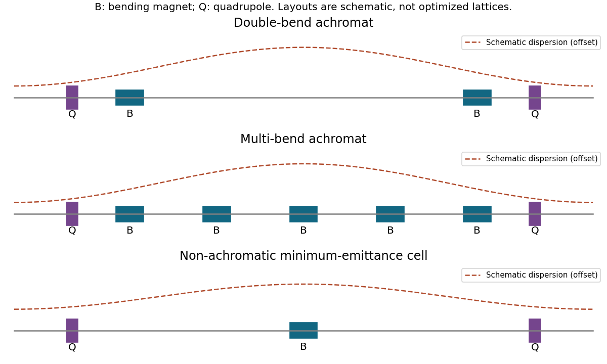
A DBA uses two bends and quadrupoles to return dispersion and its slope to zero at the cell boundaries; this provides dispersion-free insertion straights, at some emittance cost. A multi-bend achromat distributes the total angle over more weak bends and carefully controls the interior dispersion. A non-achromatic theoretical-minimum-emittance cell permits nonzero boundary dispersion and chooses the beta function and dispersion near a bend's optimum; longitudinal-gradient or reverse bends offer further control of radiation integrals. Strong focusing and dispersion suppression can increase natural chromaticity and sextupole demands, compromising dynamic aperture and momentum acceptance.

In the cold underdense model, $1-v_g/c\simeq n/(2n_c)$ and ${\gamma }_{\varphi }^2\simeq n_c/n=500$. A relativistic electron slips through half an accelerating sinusoidal wavelength over $L_d\simeq {\gamma }_{\varphi }^2{\lambda }_p\simeq 8.35$ mm. For $E_z=E_0\sin \varphi$ and injection at the start of that half-cycle, integration over $0<\varphi <\pi$ givesInjection at the field crest and acceleration only to its next zero gives half this value, about 0.51 GeV; this explains a common factor-two convention in dephasing estimates. Multiplying the peak field by the entire dephasing length is instead an upper bound, not the sinusoid's actual integral. These are ideal wave-amplitude estimates: $a_0<1$ need not excite $E_0$, and finite pump depletion, pulse evolution and injection physics may reduce the gain. Without a specified nonlinear wake shape, the data warrant an order-GeV cold-wave upper scale, not a unique precision maximum for an actual experiment.

Hydrostatic balance and the ideal gas law give $dp/dz=-pg/(R_{a}T)$, hence approximately $p=p_0{e}^{-z/H}$ with $H=R_{a}T/g$ for weak temperature variation. For well-mixed absorber abundance, ${\rho }_{\mathrm{abs}}\propto p/T$, while pressure broadening gives $k\propto p$. Thus $k{\rho }_{\mathrm{abs}}\propto e^{-2z/H}$ and its integral above height $z$ has the same scale. ThereforeThe factor two depends on both pressure dependence of absorption and constant mixing ratio; it is not the ordinary density scale height.

For constant marginal annual damage $D^{\prime }$ and positive discount rate $r$, use the Laplace transform of the preceding equations:The approximation uses $r\ll b_1$ but does not require choosing an order between $r$ and $k$. At zero discount rate the integral diverges in this model because the pulse leaves permanent positive warming and damages remain constant per degree.

The age difference is the difference between proper times along two worldlines joining the same departure and reunion events. In the inertial Earth frame a traveler who spends total coordinate time $T$ moving at speed magnitude $v$, with negligible-duration turnaround, accumulates $T\sqrt{1-v^2/c^2}$ while the stay-at-home clock accumulates $T$. These are invariant readings at reunion. Acceleration permits the change of traveling inertial frame, but the result is determined by the whole path, not a universal rule that acceleration itself slows clocks.

Relativity of simultaneity is important when explaining the same result using the traveler's successive inertial coordinates. At the turnaround, the traveler changes which distant Earth event is assigned the same time. The simultaneity slice changes, producing a jump in the coordinate time attributed to Earth in the ideal instantaneous limit. On each long inertial leg the traveler can assign a slow rate to the distant Earth clock without contradicting Earth's larger total elapsed time, because those assignments do not cover the reunion comparison with a single simultaneity convention.

The key distinction is between explaining a coordinate-based apparent symmetry and deriving an invariant result. One can calculate both proper-time integrals in one inertial frame without ever using the traveler's simultaneity jump. Conversely, claiming that each twin must simply see the other younger confuses two reciprocal comparisons between different sets of simultaneous distant events. Radar signals and Doppler shifts provide an operational account with finite signal travel times and the same reunion readings.

Thus relativity of simultaneity resolves a specific misleading inference in the paradox, but is not an extra physical mechanism that changes a clock at a distance. The worldline asymmetry and the invariant proper-time calculation suffice for the prediction; simultaneity explains why reciprocal inertial time-dilation statements cannot be pasted together indiscriminately.^[ref]

Axisymmetry supplies conserved $p_{\theta }$ in addition to conserved energy. Consequently $\boxed{f=F(H,p_{\theta })}$ is a more general stationary solution, since both arguments are constant on every trajectory. Additional independent integrals may permit still more general distributions. This is a sufficient construction, not a claim that every stationary distribution must have exactly these two arguments.

A branch point is a point around which analytic continuation changes the value of a multivalued function. For $z^{1/2}=r^{1/2}{e}^{i\theta /2}$, one circuit around zero changes the sign. A branch cut removes paths producing this ambiguity; for example $-\pi <\arg z<\pi$ gives a single holomorphic square root off the nonpositive real axis. The position of a cut is a convention, while the branch point is intrinsic.

Set $q(z)=(z-1)/(z+1)$. For $z$ outside the closed segment joining $-1$ to $1$, $q(z)$ avoids the nonpositive real axis. Therefore the principal square root of $q$ defines a holomorphic function there, with the normalization $f(\infty )=1$. The endpoints are branch points. Expanding at infinity,For a positively oriented contour surrounding the cut, its integral equals the integral on a sufficiently large positively oriented circle, since the intervening annulus is holomorphic. ThusOn the upper and lower banks, $f_{+}(x)=+i\sqrt{(1-x)/(1+x)}$ and $f_{-}(x)=-i\sqrt{(1-x)/(1+x)}$. The upper bank is traversed from $1$ to $-1$, and the lower bank from $-1$ to $1$. Their sum is $-2i$ times the required real integral. Small endpoint arcs vanish because their singularities have exponent less than one. ConsequentlyFor $\alpha =1/n$, use $f_{\alpha }=q^{\alpha }$ with the same normalization. Its expansion is $1-2\alpha /z+O(z^{-2})$, and its bank values are $e^{\pm i\pi \alpha }[(1-x)/(1+x){]}^{\alpha }$. Equating the contour integral $-4\pi i\alpha$ with $-2i\sin (\pi \alpha )$ times the real integral givesThe condition $n\ge 2$ ensures endpoint integrability. Choosing the other square-root branch reverses $I_{\Gamma }$, but also reverses both bank values, leaving the real integral unchanged.

Integrate $e^{iz}/z$ around an upper semicircle, indenting the origin by a small upper semicircle traversed clockwise. The integrand is holomorphic inside the indented contour. The large arc vanishes by Jordan's lemma, and the small arc contributes $-i\pi$, soTaking imaginary and real parts yieldsThe first integrand has a removable singularity at zero and its tails converge conditionally by Dirichlet test for improper integrals. The second integral needs a principal value at zero; its zero also follows from oddness with symmetric exclusion. One must not assign an ordinary convergent integral to its singularity.

Put $z=e^{i\theta }$, so $\sin \theta =(z-z^{-1})/(2i)$ and $d\theta =dz/(iz)$. The integral becomesThe poles are $-2i/3$ and $-3i/2$; only the first is inside the unit circle. The derivative of the denominator there is $12(-2i/3)+13i=5i$. The residue theorem therefore givesThere are no poles on the contour because the real denominator is at least one.

Use positive angular frequencies and abbreviate $p={\omega }_{pe}$, $b={\omega }_{ce}$. The left-handed index is $n_L^2=1-p^2/[\omega (\omega +b)]$. It is negative below its positive zero,For the right-handed mode, $n_R^2=1-p^2/[\omega (\omega -b)]$. Below the cyclotron resonance $0<\omega <b$ its denominator is negative and the index square is positive. Just above the resonance it is negative untilThis is the lossless electron-only cold-plasma model. Ions, collisions and resonance absorption matter outside its applicable range.

For a whistler with $\omega \ll b$ and $p^2/(\omega b)\gg 1$,The travel time through a uniform slab is $t-t_s=Lp{\omega }^{-1/2}/(2c\sqrt{b})$. In terms of ordinary frequency,An arbitrary emission time changes the intercept, not the slope. The original figure labels a dispersion constant $D=81\pm 0.5\mathrm{H}{\mathrm{z}}^{1/2}\mathrm{s}$: it is the reciprocal of the plotted slope, not the slope itself. ThereforeFor $B=80$ nT and $L=6.0\times 10^7$ m this gives $b\simeq 1.41\times 10^4{\mathrm{s}}^{-1}$, $p\simeq 2.41\times 10^5{\mathrm{s}}^{-1}$, andThe resulting forbidden right-handed frequency width isThe lower edge is about $2.24$ kHz and the upper edge about $39.5$ kHz. In the real nonuniform plasma, the travel-time coefficient measures a path integral proportional to $\int {\omega }_{pe}/\sqrt{{\omega }_{ce}}ds$. The inferred density is consequently an effective uniform-slab estimate, not a unique local density at the spacecraft. Uncertainty in the path and magnetic field likely exceeds the formal error in $D$.

Replace the slowly varying interior wave by $C$ and $e^{ik|x-x^{\prime }|}$ by one when both arguments lie within the range. The integral equation givesHenceThe integrated strength has dimensions of energy times length. For $U=-\alpha \delta (x)$, $\gamma =-\alpha$ and this is exactly the result in part c. For a regular weak potential the approximation sums the important ratio $m\gamma /(k{\hslash }^2)$ without requiring it to be small, which is why it remains useful beyond the naive first Born expansion at small momentum.

Let $\lambda =m{U}_0{a}^2/{\hslash }^2\ll 1$ and $ka\ll 1$. Inside a region of size $a$, the Schrödinger equation estimates the curvature as $a^2{\psi }^{\prime \prime }=O(\lambda +(ka{)}^2)\psi$. Matching to the incoming and reflected waves constrains the slope as well. To leading order the interior wave has nearly constant value $C$, while its small accumulated derivative change encodes the potential's integrated strength.

This is not a Born assumption that $C$ is close to one. At very low $k$ the wave can be strongly reflected even by a weak potential, and $C$ can be small. The matching solution in the next part gives $C\sim k/(k+im\gamma /{\hslash }^2)$. It implies a fractional variation across the range of order $ka+m|\gamma |a/{\hslash }^2$, which is small under the two specified conditions. ThusThe approximation requires a finite short-range potential with a controlled width and integral; it does not describe arbitrary long-range tails.

For a nonzero everywhere attractive weak potential, $\gamma <0$, the pole has $k=i\kappa$ with $\kappa =m|\gamma |/{\hslash }^2>0$. The exterior waves decay as $e^{-\kappa |x|}$, giving one shallow bound state to leading weak-coupling order:Its size ${\kappa }^{-1}$ is much larger than the potential range because $\kappa a=O(\lambda )\ll 1$. For an everywhere repulsive potential there is no negative-energy normalizable bound state: the kinetic and potential quadratic forms are both nonnegative. Its lower-half-plane pole is a virtual state, not a stable bound state. More complicated sign-changing potentials with a vanishing integral require higher-order analysis and are not covered by this simple leading result.

Factorizing the projector found in part b gives the normalized eigenfunctionswith zero continuation outside. Their squared integrals are one and different positive integers give orthogonal functions. These are the familiar infinite-square-well states shifted so that the well centre is at zero. Each eigenfunction has an arbitrary overall constant phase, which cancels from the projector.

For $E<0$, inversion of the free operator gives $G_0(x,y)=m{e}^{-\kappa |x-y|}/(\kappa {\hslash }^2)$, with $\kappa =\sqrt{-2mE}/\hslash$. The bound-state equation is $\psi =-G_{0}U\psi$, henceFor the separable kernel $V(y,z)=-\alpha F(y)F^{\ast }(z)$, defineThenAn overall normalization still has to be chosen after finding a permitted energy. A nontrivial bound state must have $C\ne 0$: if $C=0$, the potential acts as zero and a square-integrable negative-energy free solution on the whole line cannot exist. Decay or square-integrability assumptions on $F$ are needed to make these integrals well defined; smoothness alone would not ensure convergence.