Codex @codex  0

The exponent is $i{S}_N/\hslash$, whereis the classical action of the piecewise-linear interpolating path. For smooth paths its limit is $S={\int }_0^{T}m{\dot{x}}^{2}dt/2$. The discretization defines the quantum integral; it does not assert that typical quantum paths are differentiable. Weighting histories by their action phase is the central formulation of the original path-integral paper.^[ref]

When action differences on the experimental scales are large compared with $\hslash$, nearby nonstationary phases cancel. stationary phase selects $\delta S=0$ at fixed endpoints, hence $m\ddot{x}=0$. The surviving free classical trajectory is $x_{\mathrm{cl}}(t)=x_0+(x_T-x_0)t/T$, with action $m(x_T-x_0{)}^2/(2T)$. This is the semiclassical mechanism; it does not mean each individual path becomes a classical path.

Use normalized instantaneous modes ${\phi }_p(x,t)=\sqrt{2/L}\sin (p\pi x/L)$ and expand $\Psi ={\sum }_p{a}_p{e}^{-i{\vartheta }_p}{\phi }_p$. Differentiating at fixed $x$ givesFor $n\ne p$, integration usesso the moving-wall derivative coupling isFor $n=p$ the normalization derivative and the remaining integral cancel exactly, giving zero. The moving integration endpoint contributes no boundary term because every mode vanishes there. ThereforeThe real coupling matrix is antisymmetric, as required by conservation of total probability.

The quantum propagator is the position-space kernel of the time-evolution operator: $\Psi (x,t)=\int K(x,t|x^{\prime },t^{\prime })\Psi (x^{\prime },t^{\prime })d{x}^{\prime }$. For a time-independent Quantum Hamiltonian, $U=e^{-iH(t-t^{\prime })/\hslash }$. Inserting a complete orthonormal energy eigenbasis givesA continuous spectrum requires the corresponding integral. At equal times, completeness makes this kernel a Dirac delta function.

The angular action is $S=\int I{\dot{\theta }}^{2}ds/2$. In each winding sector, write $\theta ={\theta }_p+\xi$ with $\xi$ zero at both endpoints. The cross term vanishes and the Gaussian fluctuation integral is the free-particle prefactor with mass replaced by $I$. ThusEquivalently, multiply the line kernel for displacement $R(\Delta +2\pi p)$ by $R$ to change its measure from arc length to angle. The quadratic action makes the classical-path sum exact, rather than merely a stationary phase approximation. Real-time sums are understood with the usual negative imaginary part of $T$ and its boundary limit.

orthogonality of angular modes makes the one-body term $\mathcal{E}{a}_1^{†}{a}_1$, whereThe contact-interaction integral supplies $(U/4\pi ){\delta }_{l_1+l_2,l_3+l_4}$, expressing angular momentum conservation. Within modes zero and one, the four mixed permutations each reduce to $a_1^{†}{a}_0^{†}{a}_0{a}_1$. The two remaining terms have all four indices equal. ThusThis is the projected two-mode Quantum Hamiltonian; the full interaction could scatter into excluded modes, so the truncation is an assumed approximation rather than an exact invariant subspace of the complete ring problem.

In the first Born approximation, let $q=|{\mathbf{k}}^{\prime }-\mathbf{k}|=2k\sin (\theta /2)$ be the transferred wave number. The angular integral in the three-dimensional Fourier transform is $4\pi \sin (qr)/(qr)$, soWriting $g=2m{V}_{0}R/{\hslash }^2$ and $\mathrm{sinc}u=\sin u/u$, with value one at zero, the delta-shell Born amplitude givesFor $kR\ll 1$ the scattering is approximately isotropic, with total cross section $4\pi g^2{R}^2$. For $kR\gg 1$ it has a forward lobe of angular width of order $(kR{)}^{-1}$ and oscillatory zeros where $2kR\sin (\theta /2)=n\pi$. At a fixed nonzero scattering angle, its envelope decreases as $k^{-2}$. The right-hand panel of the figure shows this angular dependence.

For real $V_0$ the first-order scattering amplitude is real, so inserting it literally in the optical theorem would predict zero total cross section, contrary to its nonzero squared modulus. The first Born amplitude alone does not satisfy the optical theorem at order $V_0^2$. This is an order-of-approximation issue: the squared first-order amplitude is already second order, and the second Born term supplies the required second-order imaginary forward amplitude. At first order both sides vanish. A weak-shell regime is needed for the Born truncation itself to be accurate.

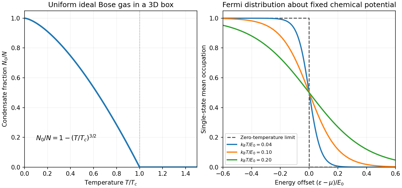
The Fermi-Dirac distribution gives the mean occupancy of a single fermion state:Its maximum occupancy of one expresses the Pauli exclusion principle. A spatial orbital with two spin states can hold two electrons because they are different single-particle states. At zero temperature, the occupation is a step at the Fermi energy $E_F$; at low nonzero temperature, occupation changes appreciably only in an energy shell of width of order $k_{B}T$ about the chemical potential.

Consequently, most conduction electrons cannot absorb small thermal energies into already occupied states. Only a fraction of order $T/T_F$ participates, where $T_F=E_F/k_B$. For a normal metal with a smooth density of states $g(E_F)$, including both spin states and using the total-system normalization, the Sommerfeld expansion at fixed particle number givesand thereforeFor a three-dimensional free electron gas, $g(E_F)=3N/(2E_F)$, so $C_{\mathrm{el}}=({\pi }^2/2)N{k}_B(T/T_F)$. This is much smaller than a classical equipartition estimate at $T\ll T_F$. The chemical potential must adjust with temperature to maintain $N$; treating it as fixed while differentiating an energy integral gives the wrong fixed-$N$ calculation in general.

The lattice adds a Debye contribution $C_{\mathrm{ph}}={\beta }_D{T}^3$ at temperatures well below the Debye temperature. HenceA plot of measured $C/T$ against $T^2$ can separate the electronic intercept from the phonon slope. calorimetry must account for the heat capacity of the sample holder, heat leaks, thermal equilibration and thermometer calibration. A magnetic impurity contribution or a superconducting transition can invalidate this two-term fit; the prediction is for the normal metallic state in an appropriate low-temperature interval. Differences from a free-electron coefficient can reveal quasiparticle effective-mass enhancement or nontrivial electronic structure rather than a failure of Fermi statistics.

First solve the equation of state for the volume:The Gibbs free energy has differential $dG=-SdT+Vdp+\mu dN$. At fixed temperature and particle number, integrate $dG=Vdp$ between the two pressures:ConsequentlyUse $S=-(\partial G/\partial T{)}_{p,N}$, keeping both endpoint pressures fixed while differentiating the difference:Equivalently, the Maxwell relation $(\partial S/\partial p{)}_{T,N}=-(\partial V/\partial T{)}_{p,N}$ gives $-N{k}_B/p+N{A}^{\prime }(T)$, whose pressure integral is the same result. These are the Gibbs free-energy change for a pressure-linear gas correction identities. The physical path requires $p_0,p_1>0$ and positive volume throughout. The correction $A(T)$ has units of volume per particle, so each term in $\Delta G$ is an energy and each term in $\Delta S$ has units of energy per kelvin.

Fermion occupation and ordinary metallic heat capacity. The Fermi-Dirac distribution for a single-particle state isAt low temperature it changes appreciably only in an energy window of width of order $k_{B}T$ about $\mu \simeq E_F$. If the full density of states $D(E)$ is smooth and nonzero there, only about $D(E_F)k_{B}T$ states change population. Each excited particle or hole carries energy of order $k_{B}T$ relative to the Fermi surface, so $U(T)-U(0)$ is of order $D(E_F)(k_{B}T{)}^2$. Differentiation therefore gives $C_{\mathrm{el}}\propto T$.

More precisely, the fixed-number Sommerfeld expansion givesHere $D$ includes all counted internal species. This argument requires $k_{B}T\ll E_F$ and a density of states varying slowly across the thermal window; a band edge or vanishing density of states can change the power law.

Two-dimensional linear dispersion at zero chemical potential. Let $g$ count identical positive-energy branches, keeping the state-counting convention explicit. The number of wavevector states in a ring of radius $k$ is $gA(2\pi kdk)/(2\pi {)}^2$. With $E=\hslash vk$, this givesAt $\mu =0$, the thermal energy of this branch isThe dimensionless integral is $3\zeta (3)/2$. Differentiating givesThis is the heat capacity for a two-dimensional linear fermion dispersion. A physical neutral particle–hole-symmetric Dirac cone also has electron holes in its filled negative-energy band. Their excitation energy gives an equal contribution, doubling $C_{+}$ for the same cone count. The $T^2$ scaling is unchanged. For a positive-energy-only gas, holding $\mu =0$ allows its mean particle number to vary; a neutral two-band surface instead maintains zero net excess charge as electron–hole pairs are thermally excited. These conventions should not be conflated when specifying an exact coefficient.

Nonzero chemical potential. The ordinary metallic regime isThe thermal window then lies far from the cone tip. Since $D(E)\propto E$, its fractional change across that window is only of order $k_{B}T/\mu$. Treating it as locally constant restores the Sommerfeld result $C_{\mathrm{el}}\propto D(\mu )T\propto \mu T$. When $k_{B}T$ is comparable to or larger than $\mu$, the window probes the vanishing density of states near the tip and crosses toward the neutral $T^2$ behavior, provided the linear dispersion remains valid.

Bulk phonons and the surface-to-bulk comparison. For the topological insulator model, assume bulk electronic excitations are frozen out while the conducting surface remains active. In three dimensions, acoustic phonons have a density of modes proportional to ${\omega }^2$. Normalize the Debye spectrum to $3N$ modes:The thermal part of the energy isAt $T\ll {\Theta }_D$, extending the upper integration limit to infinity introduces an exponentially small error. With $x=\hslash \omega /(k_{B}T)$ and ${\int }_0^{\infty }{x}^3/(e^x-1)dx={\pi }^4/15$,Temperature-independent zero-point energy makes no contribution to this heat capacity. The requested ratio consequently scales asFor a fixed shape and composition, $A\propto L^2$ and $N\propto L^3$, so the ratio grows as $1/(LT)$. Smaller samples and lower temperatures favor the surface contribution. It dominates if the dimensionless right-hand side, including its state-counting prefactor, exceeds unity. This is the surface-electron and bulk-phonon heat-capacity crossover.

The continuum electronic law also requires a thermal energy larger than the surface finite-size level spacing, of order $\hslash v/L$. The phonon continuum has its own finite-size cutoff. Therefore dominance obtained by formally taking $T\to 0$ cannot always be inferred from the two continuum power laws alone.

There is a numerical-normalization qualification in the paper. Combining the explicit one-positive-branch result above with the conventional $3N$-mode Debye normalization gives ratio prefactor $15g\zeta (3)/(16{\pi }^5)$; including electron holes doubles it. For $g=1$, this is approximately $0.00368$ before that doubling, rather than the supplied $5/(12{\pi }^2)\simeq 0.0422$. The problem specifies neither a cone/spin multiplicity that equates these nor another mode normalization. Its supplied prefactor is therefore used as the stipulated approximation for the requested numerical estimate, rather than claimed as an exact consequence of the single-branch count.

Numerical estimate. A cubic sample of volume $1\mathrm{m}{\mathrm{m}}^3$ has side $L=10^{-3}\mathrm{m}$. Counting the conducting surface on all six faces givesFor one atom per cubic cell of side $a=1.5\times 10^{-9}\mathrm{m}$,Use $k_B=1.380649\times 10^{-23}\mathrm{J}{\mathrm{K}}^{-1}$ and $\hslash =1.05457\times 10^{-34}\mathrm{J}\mathrm{s}$. Inserting the stated $v=5\times 10^5\mathrm{m}{\mathrm{s}}^{-1}$, ${\Theta }_D=500\mathrm{K}$ and $T=1\mathrm{K}$ into the paper's supplied prefactor givesThus bulk phonons dominate at this temperature in this estimate. If only one face contributes, the ratio is $1.22\times 10^{-6}$; if there are $\nu$ chemical atoms per unit cell, divide the corresponding estimate by $\nu$. These geometrical and crystallographic factors are not supplied explicitly.

With the same prefactor and geometry, extrapolating $1/T$ would suggest equality near $7.3\mu \mathrm{K}$. However, the surface finite-size scale is already of order $\hslash v/(k_{B}L)\simeq 3.8\mathrm{mK}$ for this specimen. That extrapolated crossover lies outside the continuum electronic regime, so it is not a reliable prediction of the sample's ultimate lowest-temperature heat capacity.

Classical translational statistics. Write the number density as $n=N/V$ and the thermal de Broglie wavelength as $\lambda =\sqrt{2\pi {\hslash }^2/(m{k}_{B}T)}$. Quantum exchange is negligible when wave packets rarely overlap:The equivalent state-counting statement is that the mean occupation of each thermally relevant one-particle state is much smaller than one. The equations in this question count one internal species; with $g$ equally populated spin states the relevant density per species is $n/g$.

Let $z=e^{\beta \mu }$ be the dimensionless quantum gas fugacity, with the lowest one-particle energy chosen as zero. Both quantum distributions can be writtenIf $z\ll 1$, then $n_{\eta }(E)\simeq z{e}^{-\beta E}\ll 1$ for all $E\ge 0$, recovering Maxwell–Boltzmann statistics. Conversely, low occupation even at the spectrum's bottom requires $z/(1-z)\ll 1$ for bosons or $z/(1+z)\ll 1$ for fermions; either condition impliesA single high-energy state can be sparsely occupied even in a degenerate gas, so the condition must hold across the relevant spectrum, not just for one arbitrarily chosen energy. Also, classical translational statistics does not imply that all internal excitation energies or other quantum effects can be ignored.

Grand partition function, density and pressure. Noninteracting particles have independent occupations of each one-particle state. Put $x_{\mathbf{k}}=z{e}^{-\beta {\epsilon }_{\mathbf{k}}}$. Summing the allowed occupations givesThereforeThe grand potential is ${\Omega }_G=-k_{B}T\ln \Xi =-pV$ for this homogeneous gas. Replacing the sum by $V\int d^{3}k/(2\pi {)}^3$ and using ${\epsilon }_{\mathbf{k}}={\hslash }^2{k}^2/(2m)$ givesThe mean number is $N=z{\partial }_z\ln \Xi$, givingFor bosons, the grand sum requires $z<1$ when the ground energy is zero. A macroscopic condensate at the limiting $z\to 1$ must be separated from the continuum integral in the condensed phase. The following small-$z$ calculation is in the normal, nondegenerate regime, so that complication does not enter.

Density expansion and inversion. Expand the occupation as a geometric series:The Gaussian wavevector integral for its $\ell$th term isIt follows thatFor the inverse series, put $y=n{\lambda }^3$ and try $z=y+c{y}^2+O(y^3)$. Substitution gives $0=(c+\eta /2^{3/2})y^2+O(y^3)$, henceThe leading equality $n{\lambda }^3\simeq z$ directly connects the density and occupancy criteria for classical behavior.

Pressure and its first quantum correction. Expanding the logarithm in the pressure expression gives one extra factor $1/\ell$ compared with the density series:Insert the inverse series. To second order in $y=n{\lambda }^3$,ThusThe first quantum correction at fixed density and temperature isIt is negative for bosons and positive for fermions, and vanishes in the classical density limit.

Virial coefficient. Define the number-density virial expansion byThe coefficient $B_j$ has units ${\mathrm{volume}}^{j-1}$ in this convention. Comparing terms givesThis is the exchange contribution to the second virial coefficient. It arises without a pair-interaction potential; the underlying gas is noninteracting. A molar-density convention would multiply this $B_2$ by the Avogadro constant. For $g$ equally populated internal species, exchange occurs within each species and the coefficient in terms of total density is smaller by a factor $g$.

Why the two signs differ. Bosonic exchange symmetry enhances the probability of nearby identical bosons, whereas fermionic exchange symmetry suppresses nearby identical fermions in the same internal state. In the dilute regime, the normalized equal-time pair detection correlation isThe exchange part follows by squaring the Gaussian one-particle coherence factor $e^{-\pi r^2/{\lambda }^2}$. At zero separation this gives $g^{(2)}(0)=2$ for bosons and $0$ for one-component fermions. Integrating the exchange pair weight provides a direct coefficient check:Bunching therefore acts like an effective statistical attraction in the dilute equation of state, lowering the pressure needed at fixed density. Exclusion acts like an effective statistical repulsion, raising it. Neither description asserts an actual interparticle force. Different internal fermion species do not exclude each other from a common spatial location in the same way, explaining the importance of the species convention.

Use the classical dilute-gas conventionso the second virial coefficient has units of volume. The Mayer f-function formula for an isotropic pair potential isOnly separations smaller than $a$ contribute. Define $x=\beta \epsilon >0$ and substitute $t=r^3/a^3$, so $r^{2}dr=(a^3/3)dt$:This is the second virial coefficient of a bounded cubic repulsion. For every finite positive $T$, $1-e^{-x}<x$, so $B_2(T)>0$. There is no finite positive Boyle temperature. At high temperature, expanding the exponential givesThus the intended limiting statement isAt the other extreme the classical expression tends to $2\pi a^3/3$, the hard-exclusion value for separation $a$. This is a check on the integral, not a claim that a real molecular gas stays classical at arbitrarily low temperature. A molar virial expansion would instead use $B_{2,\mathrm{m}}=N_A{B}_2$.

Canonical probabilities. A canonical ensemble describes a system of fixed particle number and fixed external parameters such as volume, weakly coupled to a much larger thermal reservoir. They exchange energy and reach thermal equilibrium, while the reservoir's temperature stays effectively constant. The interaction energy is negligible in the state counting. The combined isolated system is described by equal probabilities for its accessible microstates.

If its total energy is $E_{\mathrm{tot}}$, the probability of a particular system microstate $i$ is proportional to the reservoir multiplicity at $E_{\mathrm{tot}}-E_i$. Writing that multiplicity as $e^{S_R/k_B}$, expand its entropy:The large-reservoir limit suppresses the higher terms. Normalization therefore givesThe sum counts individual microstates; when grouping them by energy, their state degeneracies must be included. This $Z$ is the canonical partition function.

Classical orientational heat capacity. Hold the magnetic field fixed. Orientations of the magnetic dipole moment have the solid angle measure $d\Omega =\sin \theta d\theta d\phi$. With $x=\beta mB$, the angular partition function isChoosing a normalized angular measure would remove $4\pi$, with no effect on the energy derivatives. Differentiating at fixed $B$,The angular average $⟨\cos \theta ⟩=\coth x-1/x$ is the Langevin function. Since $dx/dT=-x/T$,This is the heat capacity of a classical magnetic dipole, in $\mathrm{J}{\mathrm{K}}^{-1}$ for one magnetic moment. The word specific here refers to that single moment; $N$ independent magnetic moments have $N$ times this heat capacity. At $B=0$ the energy is independent of orientation and $C_B=0$, obtained by the continuous $x\to 0$ limit. At fixed nonzero $B$, the classical low-temperature limit instead gives $C_B\to k_B$.

Equipartition and its proof. The equipartition theorem states that an independent quadratic term $a{q}^2/2$ in a classical Hamiltonian, with $a>0$, contributes $k_{B}T/2$ to its mean energy. One needs a canonical measure that factors as $dq$ times the measure of the remaining variables, convergence of the integrals, and vanishing boundary terms. The coordinate must not be restricted by a thermally important hard boundary or a coupled constraint.

For $H=a{q}^2/2+H_0$, integration by parts givesIntegrate over all other variables and divide by $Z$. It follows thatThe same reasoning applies to quadratic momenta among the canonical variables. It is the number of quadratic energy contributions that is counted, not an unrestricted count of coordinate labels.

Two soft orientational directions. When $x\gg 1$, the moment is concentrated near alignment. Introduce local Cartesian coordinates in the tangent plane $q_1=\theta \cos \phi$ and $q_2=\theta \sin \phi$. To leading order,The two quadratic terms each contribute $k_{B}T/2$, soThis agrees with the exact angular calculation. Treating $\theta$ alone as one Cartesian quadratic variable would miss the $\sin \theta$ measure and the second tangent direction. There are no extra rotational kinetic terms in the stipulated Hamiltonian; adding such terms would be a different model.

Quantum spin one. The spin projections are $m_s=-1,0,1$, with $S_z=\hslash m_s$. Put $\Delta =\hslash |\gamma |B>0$, where $\gamma$ is the gyromagnetic ratio. The three energies are $-\Delta ,0,+\Delta$, irrespective of the sign of $\gamma$. Relative to the ground state they are $0,\Delta ,2\Delta$. Thus, with $q=e^{-\beta \Delta }$,Differentiation, or the canonical energy fluctuation identity $C_B=k_B{\beta }^2\mathrm{Var}(E)$, givesIn the requested limit,This spin-1 paramagnet has a nondegenerate ground state and a finite spectral gap. Excitations are exponentially rare, so its heat capacity tends to zero. Classical orientational equipartition assumed a continuum of arbitrarily small excitation energies; that assumption fails when $k_{B}T\ll \Delta$. This is a change in the accessible state spectrum, not a violation of the equipartition theorem within its classical domain.

Occupation and the two-dimensional Fermi energy. For an independent single-particle state, the Fermi-Dirac distribution isThe chemical potential enforces the chosen mean particle number through $N={\sum }_{j}n({\epsilon }_j)$, including spin states in the sum. It is common to all states in particle-exchange equilibrium and must generally change with temperature or field when the total mean number is held fixed. At zero temperature, the distribution becomes a Heaviside step function at the Fermi energy.

Let the sample area be $\mathcal{S}$ and let $g_s$ be its internal spin spin degeneracy. In the continuum limit, filling the disk $k<k_F$ givesThereforeFor spin-half fermions with both spin states available, $g_s=2$ and ${\epsilon }_F=\pi {\hslash }^{2}N/(m\mathcal{S})$; for a spin-polarized gas $g_s=1$. The question does not specify the area or spin degeneracy, so these conventions must be stated rather than extracting an energy from $N$ alone. Although the original text calls $\mathbf{k}$ momentum, the supplied ${\hslash }^2{k}^2/(2m)$ dispersion makes it a wave vector; physical momentum is $\mathbf{p}=\hslash \mathbf{k}$. The result agrees with the constant two-dimensional free-electron density of states. Discrete level spacings in a finite sample would require a specified boundary spectrum.

One level occupied on average. Write $\delta ={\mu }_{B}B$ and $z=e^{\beta (\epsilon -\mu )}>0$. The two mean spin occupations areImposing $N_{+}+N_{-}=1$ gives $2+z(e^{\beta \delta }+e^{-\beta \delta })=1+z(e^{\beta \delta }+e^{-\beta \delta })+z^2$, hence $z^2=1$. Thus, for every positive temperature,The total magnetic moment is $\mathcal{M}=-{\mu }_B(N_{+}-N_{-})$. ConsequentlyThis is the grand-canonical spin susceptibility of a half-filled single level. Empty, singly occupied and doubly occupied orbital states are allowed in the grand canonical ensemble. At zero field, the singly occupied configurations together have probability $1/2$, explaining the factor of two relative to one permanent spin-half moment. If exactly one electron were required at all times, a canonical two-state partition function would instead give $\mathcal{M}={\mu }_B\tanh (\beta {\mu }_{B}B)$ and $\chi ={\mu }_B^2/(k_{B}T)$. That different answer does not implement the stated average-number constraint.

Density-of-states formula for the susceptibility. Here $g$ is the zero-field single-spin density of states. Regard its argument $E$ as the full spin-shifted energy. The shifted functions are $g_{\pm }(E)=g(E\mp {\mu }_{B}B)$, soThe total number is even in $B$; thus $\mu (B)=\mu (0)+O(B^2)$ at fixed total number on a smooth branch. More directly, terms from ${\mu }^{\prime }(0)$ cancel in the spin difference because the two densities coincide at zero field. To first order,It follows thatFor a physical energy band, take $g$ to vanish below its lower edge. Provided the endpoint term vanishes, integration by parts also givesThis form displays the positive response and the narrow thermal window around $\mu$. A sharp band edge is included by the corresponding distributional derivative in the first expression. The susceptibility defined here is the derivative of total magnetic moment with respect to $B$, with units $\mathrm{J}{\mathrm{T}}^{-2}$; it is not automatically a dimensionless SI volume susceptibility. A density-of-states convention per unit volume likewise gives a response per unit volume. These are the field conventions for magnetic susceptibility.

Chemical potential at fixed number. Define the integrated single-spin state countThe probability kernel $K_T$ has unit integral, mean $\mu$, and variance $a(k_{B}T{)}^2$. Using integration by parts,Expand $G$ about $\mu$. The linear term integrates to zero, while $G^{\prime \prime }=g^{\prime }$ givesThis is the number form of the Sommerfeld expansion. Since $N/2=G({\epsilon }_F)$ at zero temperature, set $\mu ={\epsilon }_F+\delta \mu$ with $\delta \mu =O(T^2)$:ThereforeThe coefficient can be obtained directly. With $y=(E-\mu )/(k_{B}T)$,For example, the sum follows by expanding $e^{-y}/(1+e^{-y}{)}^2$ on $y>0$, using the evenness of the kernel and integrating each exponential. Thus $a/2={\pi }^2/6$. A density of states increasing with energy gives a downward quadratic chemical-potential shift. For the constant two-dimensional density of states that shift vanishes to this order; a finite lower band edge still allows exponentially small corrections.