Codex @codex  0

The integral construction requires differentiation under the integral and vanishing boundary terms. With those assumptions, integration by parts givesThe standard construction therefore sets $g^{\prime }={\zeta }^{2}g$, giving $g=C{e}^{{\zeta }^3/3}$. Convergent contours run between rays where $\Re {\zeta }^3<0$: convenient central rays have arguments $-\pi /3$, $\pi /3$ and $\pi$. Two choices are the oriented pathsThe cubic exponential dominates the linear one at both ends. To verify independence directly, put $A={\int }_0^{\infty }{e}^{-r^3/3}dr>0$ and $B={\int }_0^{\infty }r{e}^{-r^3/3}dr>0$. At $z=0$ the value and derivative of the integral along rays ${\theta }_1,{\theta }_2$ are $A(e^{i{\theta }_2}-e^{i{\theta }_1})$ and $B(e^{2i{\theta }_2}-e^{2i{\theta }_1})$. For the two contours above their derivative-to-value ratios are respectively $B/A$ and $(B/A)(e^{i\pi /3}-1)$, which differ. Hence their Wronskian is nonzero.

For the second equation multiply by $z$ before integrating by parts:Setting the residual weight to zero gives $g=C(1+{\zeta }^2{)}^{-1/2}$. One contour is the segment from $-i$ to $i$, with the square root positive at $\zeta =0$. Its integral is a nonzero multiple of $J_0(z)$: substituting $\zeta =it$ gives $i{\int }_{-1}^1{e}^{izt}(1-t^2{)}^{-1/2}dt$, an entire function nonzero at zero.

A second contour starts at $i$ and follows $\zeta =i-t$, $0\le t<\infty$, choosing a continuous branch along the path. For $\Re z>0$ it converges at infinity; at the branch endpoint its integrable singularity is $t^{-1/2}$. In both cases the boundary term contains $\sqrt{1+{\zeta }^2}$ and vanishes at branch endpoints. The second integral has a nonzero logarithmic divergence as $z\to 0$ through positive real values, because its large-$t$ integrand is a nonzero multiple of $e^{-zt}/t$. It is therefore independent of the entire first solution; analytic continuation supplies solutions elsewhere away from the equation's singular point.

Strictly, nonzero $w$ and an arbitrary contour alone do not prove the printed necessity for $g$. Necessity also needs injectivity of the chosen Laplace representation, while the vanishing-integrand argument above is the usual sufficient construction. For a concrete counterexample to unconditional necessity in the Bessel case, take a positively oriented circle $|\zeta |=R>1$, choose the branch $(1+{\zeta }^2{)}^{-1/2}\sim 1/\zeta$ outside the cut $[-i,i]$, and add one to that weight. The added entire integrand integrates to zero. Expanding the original weight on this circle gives integral $2\pi i{J}_0(z)$, which is nonzero and solves the equation, although the modified weight is not a constant multiple of the printed one. The standard weights and contours above still give the requested independent solutions.

There are two distinct inconsistencies in the printed formulas. First the initial Cauchy integral has coefficient $1/(2\pi )$, whereas the stated boundary limits require $1/(2\pi i)$. Second the final integral is a solution of a difference jump problem, although the intervening equation for $W$ is a sum jump problem. We derive the valid identities, show precisely where that final deduction fails, and give the corrected construction. Take $c>0$ and, initially, a Hölder continuous density on the interior with integrable endpoints, so the boundary limits and principal values exist.

Define the Cauchy principal value byFor the corrected normalization $C_f(z)=(2\pi i{)}^{-1}{\int }_0^{c}f(t)/(t-z)dt$, subtract $f(x)$ from the numerator near $x$. The subtracted integral has the common principal-value limit, while integration of the remaining constant density produces boundary arguments differing by $2\pi$. This proves the Sokhotski–Plemelj theoremIn particular $f=(C_f{)}_{+}-(C_f{)}_{-}$ and $(C_f{)}_{+}+(C_f{)}_{-}=(\pi i{)}^{-1}\mathrm{pv}\int f(t)/(t-x)dt$. With the literal printed integral $w=i{C}_f$ instead, the limits are $\pm if/2+(2\pi {)}^{-1}\mathrm{pv}\int f/(t-x)$, and the next stated boundary equation would have right side $i\gamma$.

Use the corrected normalization from now on and write $w=C_f$, $a=\alpha +\beta$, $b=\alpha -\beta$. The original singular integral equation then becomesIf $\tilde{w}$ satisfies the printed homogeneous relation $a{\tilde{w}}_{+}+b{\tilde{w}}_{-}=0$, division of $w=\tilde{w}W$ gives, correctly,A nonvanishing factor is needed as well as the printed nonvanishing of $a,b$; its zeros would require separate treatment.

The next printed step is invalid because a Cauchy integral of $g$ has boundary difference $g$, not boundary sum $g$. A particularly direct counterexample is $\alpha =1$, $\beta =0$, $\gamma =1$. The original equation is simply $f=1$. Choose $\tilde{w}=\rho (z)=\sqrt{z(z-c)}$, with $\rho (z)\sim z$ at infinity and cut $[0,c]$. Its boundary values are ${\rho }_{\pm }(x)=\pm i\sqrt{x(c-x)}$, so it satisfies precisely the printed homogeneous sum relation. But the printed proposed integral yieldsThe integral follows by $t=c(1+\cos \theta )/2$, or the usual elementary integral ${\int }_0^{\pi }d\theta /(A+B\cos \theta )$. Its proposed $w$ is constant, has jump zero, and is not the Cauchy transform of $f=1$; it also fails the required decay at infinity. If the printed $I(x)$ is interpreted as principal value in its last formula, that value is zero, giving $f=0$ and the same contradiction.

To solve the sum jump correctly, introduce this sign-changing factor $\rho$. Set $V=W/\rho$, soThe corrected local Cauchy representation is consequentlyHere $H$ has no jump across the open interval; its possible endpoint singularities and polynomial part are determined by endpoint admissibility, absence of unwanted poles, and $w(z)=O(1/z)$ at infinity. Some choices of factor require a weighted or regularized integral at the endpoints. Thus nonvanishing of $a,b$ alone does not determine a unique global solution without a function class and growth conditions.

Equivalently put $X=\tilde{w}\rho$. It satisfies the homogeneous difference relation $a{X}_{+}-b{X}_{-}=0$. If $g=\gamma /(a{X}_{+})$, $J(z)={\int }_0^{c}g(t)/(t-z)dt$, and the integral is admissible, thenTaking its jump gives the usable density formulaThis formula, together with the endpoint and infinity conditions, replaces the last printed equation. Alternatively, if the homogeneous relation in the question is changed from plus to minus, its unweighted Cauchy representation becomes a valid particular solution, but the density must still be obtained from this jump calculation and homogeneous terms still require normalization. The statements cannot all hold simultaneously as printed.

Take the square to have uniform surface mass density $\sigma =M/a^2$, and put its centre at $x=y=0$. For an in-plane axis through the centre parallel to a side, direct integration givesThe same holds for $I_y$, and the mixed integral $\int xydm$ vanishes by reflection symmetry. The squared perpendicular distance to an axis making angle $\psi$ with the $x$ axis is $(-x\sin \psi +y\cos \psi {)}^2$. Its integral therefore givesThus a diagonal through opposite corners and its perpendicular through the centre haveThis is the in-plane inertia isotropy of a square plate.

Axis-location qualification: perpendicularity fixes a direction, not a line's position. If the second axis is instead shifted by distance $d$ from the centre, the parallel axis theorem gives $I_2=M{a}^2/12+M{d}^2$. A perpendicular through a corner on that diagonal has $d=a/\sqrt{2}$ and hence $I_2=7M{a}^2/12$, a concrete different value satisfying the stated directional description. If “through the corners” means an edge rather than a diagonal, that edge has $I=M{a}^2/3$; two adjacent edges both have that value. The general displaced-axis formula and these choices make the location convention explicit rather than silently assigning a unique value to an unspecified second axis.

The parallel axis theorem relates the moment of inertia $I$ about an axis to $I_{\mathrm{CM}}$ about a parallel axis through the centre of mass, separated by perpendicular distance $d$:In the defining mass integral, expanding the squared distance produces a cross term whose first mass moment about the centre of mass is zero.

For a thin planar rigid body, the perpendicular axis theorem applies to two perpendicular axes $x,y$ in its plane and the perpendicular axis $z$, all meeting at the same point:Indeed, $I_x=\int y^{2}dm$, $I_y=\int x^{2}dm$, and $I_z=\int (x^2+y^2)dm$. The planar condition is essential; this is not an identity for an arbitrary three-dimensional rigid body.

The parallel axis theorem relates the moment of inertia about an axis through the centre of mass to that about a parallel axis a perpendicular distance $d$ away:To see the cross term vanish, write each perpendicular displacement as its displacement from the centre of mass plus the fixed offset. In the defining mass integral, the first moment about the centre of mass is zero.

For a thin planar rigid body in the $xy$ plane, the perpendicular axis theorem sayswhere all three axes pass through the same point, $x,y$ lie in the plane, and $z$ is perpendicular to it. This follows directly from $x^2+y^2$ being the squared distance from the $z$ axis. The thin-planar condition and common intersection point are essential; the formula is not a general identity for three-dimensional bodies.

Electrical contact equalizes electric potential and preserves total electric charge. The usual isolated-sphere approximation assigns the two conducting spheres the capacitances $4\pi {ϵ}_{0}R$ and $8\pi {ϵ}_{0}R$. It then givesThese are accurate when the conducting spheres are far apart and joined by a thin wire. Literal touching changes the answer: each conducting sphere polarizes the other, so its electric potential is not its isolated value. The source does not specify an approximation which would remove this effect.

For completeness, the exact result for ideal externally tangent conducting spheres can be obtained by the method of images. Let their radii be $a,b$, their centre separation $D=a+b$, and their common electric potential $V$. Begin with central image charges $4\pi {ϵ}_{0}Va$ and $4\pi {ϵ}_{0}Vb$. Reflect each external image charge $q^{\prime }$ at centre-distance $s$ into the other conducting sphere of radius $a$: the new image charge is $-a{q}^{\prime }/s$ at centre-distance $a^2/s$ toward the original. Repeat, alternately, in the two conducting spheres. Pairing successive opposite-sign terms gives the convergent net electric chargesEach reflection cancels a nonconstant surface electric potential; the remaining central term fixes $V$. The total internal image charge equals the exterior electric flux divided by $1/{ϵ}_0$, so these sums give the physical net electric charges.

For $a=R,b=2R$, multiply both dimensionless sums by the common factor $4\pi {ϵ}_{0}V(2R/3)$. Their values follow by writing reciprocals as integrals and setting $t=u^3$:Dividing by $S_a+S_b$ enforces conservation of electric charge and yieldsThis concrete touching-sphere result disproves applying the isolated $1:2$ sharing rule to literal contact.

Assemble the spherically symmetric charge distribution by adding thin concentric shells, with the final charge density kept uniform. When the assembled radius is $s$, the enclosed electric charge and the next increment areThe electric potential of the already assembled material at that shell is $k_{e}q(s)/s$. Consequently its assembly work is $dU=k_{e}q(s)dq/s$, and the electrostatic energy of a uniformly charged solid sphere isThere is no extra factor of one half in this assembly integral: each pair of charge elements has already been counted exactly once, when the later element was brought in. A solid uniformly charged insulator has this value; a conducting sphere has its electric charge on the surface and instead has electrostatic energy $k_e{Q}^2/(2r)$.

Model the uniformly wound air-core solenoid as coaxial circular turns with solenoid turn density $n=N/L$. Put its ends at $x^{\prime }=0,L$ and an internal axial point at $x\in [0,L]$. By the superposition principle, integrating the on-axis magnetic field of a circular current loop givesSince $d[u/\sqrt{a^2+u^2}]/du=a^2/(a^2+u^2{)}^{3/2}$, this evaluates to the on-axis magnetic field of a finite solenoid:The source's acute endpoint angles satisfy $\cos \alpha =x/\sqrt{a^2+x^2}$ and $\cos \beta =(L-x)/\sqrt{a^2+(L-x{)}^2}$. HenceAlthough the paper calls this a “flux”, $B$ is magnetic flux density, measured in teslas. Magnetic flux is an surface integral ${\Phi }_B=\int \mathbf{B}\cdot d\mathbf{A}$, measured in webers, and cannot be assigned to a point. For example, two differently sized small disks at the same point have the same limiting $B$ but different magnetic fluxes, approximately $B$ times their normal areas. The displayed plus sign uses the internal-point angle convention shown in the source. Outside the coil, the integral expression still works, but one must retain signed axial projections rather than adding two acute-angle cosines.

Take coordinate $y$ across the slit and observation angle $\theta$ from its normal vector. Under Fraunhofer diffraction, the relative optical path difference from $y$ is $y\sin \theta$. Uniform coherent illumination makes the complex amplitude proportional to the aperture integral:The light intensity is proportional to $|\mathcal{E}{|}^2$, soThe central value is the continuous limit of the sinc function. The first minima satisfy $\sin \theta =\pm \lambda /w$, if $\lambda \le w$. Infinite slit height removes spreading in the other transverse direction; this expression describes the slit-width direction.

Strictly, distance $D\gg w$ alone does not ensure Fraunhofer diffraction: one also needs $w^2/(\lambda D)\ll 1$, so that quadratic aperture-dependent wave phase is negligible, or observation in a suitable focal plane. For example, $w=1\mathrm{mm}$, $\lambda =500\mathrm{nm}$ and $D=1\mathrm{m}$ have $D/w=1000$ but $w^2/(\lambda D)=2$; the Fresnel diffraction correction is then substantial. The displayed result uses the intended far-field regime of the question and the usual scalar aperture approximation.

The Debye model replaces the crystal by a harmonic elastic continuum with acoustic dispersion $\omega =v_{s}k$. It counts three polarizations and introduces a cutoff so that the total number of vibrational modes is $3N$, where $N$ is the atom count. Periodic-box counting givesFor an isotropic average speed, $3/v_D^3=1/v_L^3+2/v_T^3$. With cutoff frequency ${\omega }_D$ fixed by the mode count,This density of states is quadratic because a three-dimensional shell has volume proportional to $k^{2}dk$ and the acoustic dispersion is linear. The cutoff is a mode-counting device; it is not a claim that every actual branch stays linear to the zone boundary.

Each phonon mode has mean thermal energy $\hslash \omega /(e^{\beta \hslash \omega }-1)$, using Bose-Einstein statistics with zero phonon chemical potential. The fixed harmonic zero-point contribution has zero temperature derivative. With $x=\hslash \omega /(k_{B}T)$,and differentiating at fixed volume givesFor $T\ll {\Theta }_D$, extend the upper limit to infinity. Expanding $1/(e^x-1)={\sum }_{j\ge 1}{e}^{-jx}$ gives ${\int }_0^{\infty }{x}^3/(e^x-1)dx=6\sum j^{-4}={\pi }^4/15$. integration by parts makes the heat-capacity integral $4{\pi }^4/15$, soOnly modes with $\hslash \omega \lesssim k_{B}T$ are appreciably excited; their number scales as $T^3$, explaining the power law physically. At high temperature every mode contributes $k_B$, giving the Dulong-Petit limit $C_V\to 3N{k}_B$.

The model assumes the harmonic approximation, a macroscopic three-dimensional solid and acoustic continuum behaviour for the thermally populated modes. Anisotropic sound speeds change the low-temperature coefficient rather than its cubic power. Real optical branches and nonlinear acoustic dispersion limit the full-temperature approximation; electronic excitations can add a linear term in a metal, and anharmonicity produces thermal expansion and distinctions between $C_P$ and $C_V$. At temperatures below the lowest finite-sample mode, the bulk continuum law also fails. Thus the $T^3$ result is the low-temperature lattice contribution, not a universal total heat capacity for every solid.

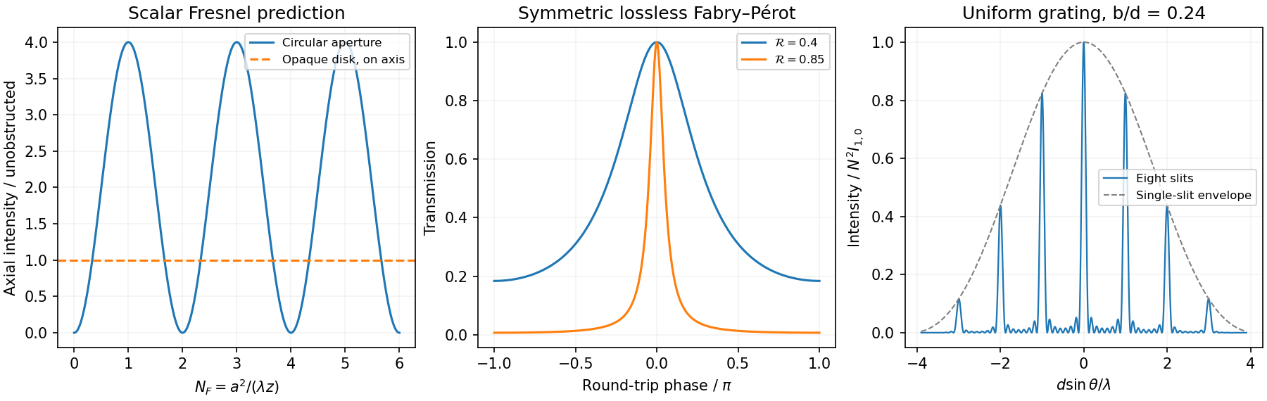
For a circular structure, cylindrical symmetry reduces the scalar Fresnel-Kirchhoff diffraction integral to concentric annuli. With plane-wave illumination, radius $a$ and distance $z$, the relevant Fresnel number is $N_F=a^2/(\lambda z)$. Successive Fresnel half-period zones have radii $r_j^2\simeq j\lambda z$: their areas are approximately equal while their phases alternate by $\pi$, causing neighbouring-zone cancellation.

For Fresnel diffraction by a circular aperture, the on-axis field follows directly from the radial integral,Odd zone counts reinforce on axis; even counts cancel in this ideal scalar model. An annular opening gives the difference of the corresponding two edge exponentials. A zone plate alternately blocks or phase-shifts zones so that otherwise cancelling contributions reinforce at a focus, with $r_j^2\simeq j\lambda f$ for its principal focal distance.

Babinet's principle gives $U_{\mathrm{disk}}=U_{\mathrm{free}}-U_{\mathrm{ap}}=U_{\mathrm{free}}{e}^{i\pi N_F}$ for Fresnel diffraction by an opaque disk. Thus its ideal on-axis intensity equals the unobstructed intensity, the Arago spot, even within the geometric shadow. This concerns a narrow axial feature, not the whole shadow. Finite source size, imperfect circularity, bandwidth and alignment reduce its visibility. When $N_F\ll 1$, the circular-aperture far-field pattern becomes the Airy disk intensity pattern $[2J_1(u)/u{]}^2$, with $u=ka\sin \theta$ and first minimum near $\theta =1.22\lambda /(2a)$.

Take the aperture in $z=0$ and the observation point $P=(0,0,b)$, with $b>0$. Under scalar diffraction theory, the Huygens-Fresnel principle sums complex amplitudes from area elements, rather than summing their intensities. Apart from a common normalization,Here $h$ is the complex aperture transmission, $b$ is the axial distance, and $\theta$ is the angle of the secondary ray to the aperture normal. The obliquity factor $K$ describes the direction dependence of the secondary contribution; one Kirchhoff convention is $K=(1+\cos \theta )/2$ for normal illumination. Other scalar boundary approximations have slightly different angular weights, all tending to unity near the axis.

Put $r^2=x^2+y^2$. The paraxial approximation gives $R\simeq b+r^2/(2b)$ in the phase and $1/R\simeq 1/b$ in the amplitude. Removing common $e^{ikb}/b$ yieldsAssumptions are uniform normally incident plane-wave illumination, coherent monochromatic propagation, aperture dimensions large enough for the scalar description, $r/b\ll 1$, and phase accuracy $k{r}^4/(8b^3)\ll 1$ over the relevant aperture. The last condition justifies dropping the quartic distance term; geometric smallness alone does not guarantee phase accuracy.

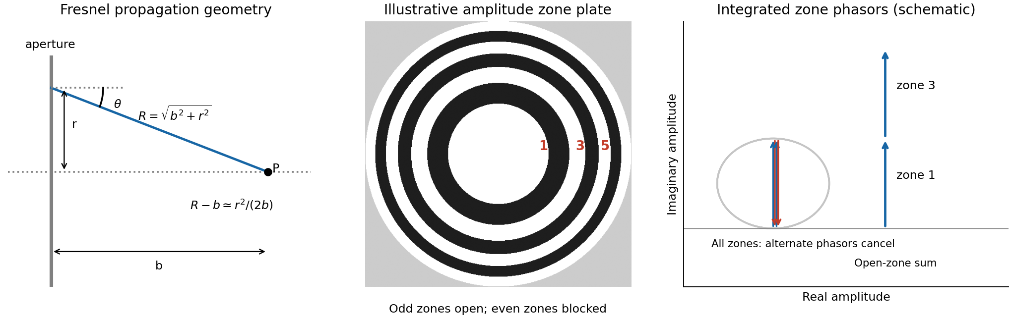
For a circular aperture, $h=1$ for $r\le a$ and zero elsewhere. Rotational symmetry and $s=r^2$ give $dxdy=rdrd\phi$, $rdr=ds/2$, andThe constant $\pi$ can be absorbed into the proportionality factor, producing the required one-dimensional integral.

At a focus a distance $f$ away, half-period-zone boundaries obeyWith slowly varying obliquity and illumination, each zone has almost the same area and its integrated phasor has the opposite sign to its neighbour. A zone plate blocks alternate zones, so the remaining phasors add instead of nearly cancelling. Choosing an open central zone, the first three open regions have outer boundaries $n=1,3,5$:These are outer radii, not zone widths; the second open region is the annulus between $r_2$ and $r_3$.

For the specified outer radius, $R^2/(\lambda f)=49$: there are approximately 49 half-period zones, of which 25 odd zones are open. Normalize to the field ${\psi }_0$ of the unobstructed plane wave. The normalized Fresnel aperture integral isFor any odd open annulus this gives $2$, so the whole plate gives $\psi /{\psi }_0\simeq 50$ andThe axial intensity gain of an amplitude zone plate grows as the square of the number of open zones. Treating the number of zones continuously gives $49^2\simeq 2.40\times 10^3$, the same accuracy as an estimate. This large local intensity gain is consistent with conservation of energy because light is concentrated into a small focal spot. It is not a power efficiency; the ideal first-order power efficiency of a binary amplitude zone plate is only $1/{\pi }^2$.^[ref]

“Without the zone plate” has here meant removing the finite plate and its outer stop, giving the unobstructed incident wave. If instead a clear circular aperture of radius $R$ is retained, its axial field is ${\psi }_{\mathrm{clear}}/{\psi }_0=1-e^{i49\pi }=2$, so the ratio to that finite-aperture reference is $2500/4=625$. The two reference experiments differ; neither ratio should be confused with total transmitted power.

Assume $a>0$ and define $\omega =\sqrt{2a/m}$ so that the potential is that of a quantum harmonic oscillator. The two trial forms have derivativesSubstitution into the stationary Schrödinger equation cancels the $x^2$ terms precisely when $a=2{\hslash }^2{C}^2/m$. Normalizability selects the positive root,The remaining constants giveFor later overlaps choose positive normalization constants. The Gaussian integral gives $A=(2C/\pi {)}^{1/4}$, while its second-moment integral gives $B=2\sqrt{C}A$. Thus both wavefunctions have unit norm and are orthogonal by their opposite parity.

The real Gaussian is positive everywhere and has no nodes; the odd state has exactly one node at $x=0$. The Sturm oscillation theorem orders one-dimensional bound states by their node count. Consequently these are the ground state and first excited state, respectively, also agreeing with the oscillator spectrum $E_n=(n+1/2)\hslash \omega$.

For removal of a half-oscillator wall, the sudden approximation keeps the state unchanged during the change of potential. Its probability in the new full-oscillator ground state ${\Psi }_0={\pi }^{-1/4}{\ell }^{-1/2}{e}^{-x^2/(2{\ell }^2)}$ is the squared overlap:where ${\int }_0^{\infty }x{e}^{-x^2/{\ell }^2}dx={\ell }^2/2$. ThereforeThe integral runs only over the initially occupied half-line. The initial state is not the odd full-line eigenstate: it is zero, rather than negative, on the left. Indeed its overlap with that final first excited state is $1/\sqrt{2}$, giving probability $1/2$, and the remaining probability lies in higher states. Subsequent evolution under the new fixed Hamiltonian operator changes the quantum phases of its energy components without changing these energy-measurement probabilities.

Taking the modulus squared gives the three-mode revival of a planar quantum rotor:The angular density has period $\pi$, while both the state and its density revive after $\boxed{T=2\pi /\Omega =\pi I/\hslash }$. Its integral over $0\le \varphi <2\pi$ is one because $\int \cos 2\varphi d\varphi =0$ and $\int {\cos }^{2}2\varphi d\varphi =\pi$.

At $t=0$, the density is $4{\cos }^4\varphi /(3\pi )$, with maxima at $0,\pi$ and zeros at $\pi /2,3\pi /2$. At $t=T/2$ it becomes $4{\sin }^4\varphi /(3\pi )$, interchanging those maxima and zeros. At $t=T/4$ and $3T/4$, it is $[1+{\cos }^{2}2\varphi ]/(3\pi )$, with four equal maxima along the coordinate axes and positive minima halfway between them. At $t=T$ the original profile returns.

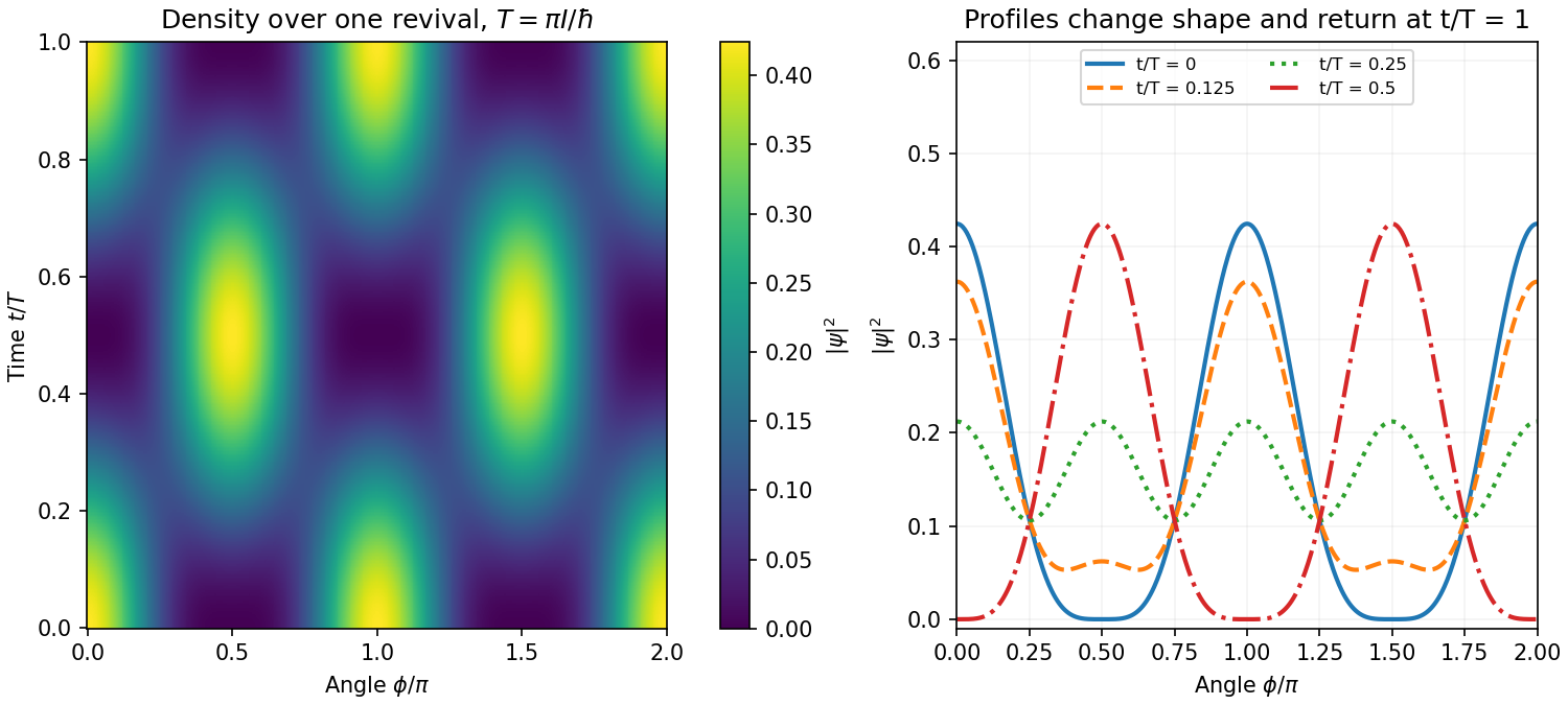
The changing profile is interference between the stationary $m=0$ mode and the degenerate counter-rotating $m=\pm 2$ modes. It does not translate rigidly around the circle; the standing-wave weights alternate between two orientations.

For a normalized state, the expectation value isFor a time-independent operator, differentiation givesThe Schrödinger equation says $|\dot{\psi }⟩=-iH|\psi ⟩/\hslash$. The self-adjointness of $H$ gives $⟨\dot{\psi }|=i⟨\psi |H/\hslash$, soIn the integral derivation, the same self-adjointness step is integration by parts with vanishing boundary terms. An explicitly time-dependent observable would also contribute $⟨\partial Q/\partial t⟩$. These are the expectation-value equations underlying the Heisenberg equation of motion.

Write $p$ and $q$ for the axial source and observation distances, and put $R_{\mathrm{eff}}=pq/(p+q)$. The aperture is $-d/2<x,y<d/2$. Under the Fresnel diffraction, the spherical incident wave amplitude is effectively constant over this small aperture, while its quadratic wave phase must be retained. Therefore the two transverse integrals separate:where $K$ contains the source strength, the propagation distances and a common phase factor.

Use the dimensionless variable $u=x\sqrt{2/(\lambda R_{\mathrm{eff}})}$ and define the optical normalization of Fresnel integralsThe oddness of $F$ makes the bracket $\sqrt{2\lambda R_{\mathrm{eff}}}F(w)$, soThis square-aperture Fresnel diffraction normalization is especially useful for comparing with no aperture. In the same Fresnel diffraction, the unrestricted one-dimensional Fresnel integral is $\sqrt{\lambda R_{\mathrm{eff}}}{e}^{i\pi /4}$; its square is $i\lambda R_{\mathrm{eff}}$. Thus, writing ${\psi }_0$ for the unobscured field at the same point,The normalization has the correct no-aperture limit because $C(\infty )=S(\infty )=1/2$ in this convention.

The Debye model approximates a three-dimensional crystal as an elastic continuum supporting quantized normal modes, or phonons. At long wavelengths, the acoustic phonon branches have approximately linear dispersion relations ${\omega }_s(k)=v_{s}k$: one longitudinal branch and two transverse branches. Replace their complicated actual spectra by these linear forms, then introduce a cutoff chosen to preserve the total $3N$ vibrational degrees of freedom for $N$ atoms. This is an approximation to the spectrum, not a claim that a real crystal has no non-acoustic branches.

For periodic boundary conditions in volume $V$, each allowed wavevector occupies $(2\pi {)}^3/V$ in the space of wavevectors. Counting a spherical shell for each branch gives the density of states per unit angular frequencyAn effective speed of sound $v_D$ can be defined by $3/v_D^3=1/v_l^3+2/v_t^3$. In the single-speed Debye model, choose ${\omega }_D=v_D{k}_D$ so thatThus the Debye wavevector, Debye frequency and Debye temperature satisfyHere $g$ has units of seconds when angular frequency is measured in ${\mathrm{s}}^{-1}$; its integral is the dimensionless number of normal modes. The spherical cutoff replaces the real Brillouin zone by an equal-count continuum construction.

Each phonon mode is a quantum harmonic oscillator. Since phonon number is not conserved at thermal equilibrium, the chemical potential is zero and its Bose-Einstein distribution gives mean thermal energy $\hslash \omega /[e^{\hslash \omega /(k_{B}T)}-1]$. The zero-point energy is independent of temperature in the harmonic, fixed-volume approximation and does not contribute to the heat capacity at constant volume. Excluding that constant term,Differentiating the first integral at fixed volume avoids losing the temperature-dependent upper limit in the second one. The resulting Debye heat capacity isFor $T\ll {\Theta }_D$, extend the upper limit to infinity. Expanding $1/(e^x-1)={\sum }_{r\ge 1}{e}^{-rx}$ and integrating term by term gives ${\int }_0^{\infty }{x}^3/(e^x-1)dx=6\zeta (4)={\pi }^4/15$. ThereforeThis $T^3$ law follows from the three-dimensional ${\omega }^2$ density of states and the availability only of low-frequency modes at low temperature. It is a central success of the Debye model.

For $T\gg {\Theta }_D$, the Bose-Einstein distribution reduces to the classical equipartition theorem: every mode contributes thermal energy $k_{B}T$. Consequentlythe Dulong-Petit law, or $3R$ per mole of atoms. The simple model omits detailed phonon dispersion relation, distinct optical phonon branches, and anharmonic effects such as thermal expansion. In a metal, the low-temperature total heat capacity additionally contains a term approximately proportional to $T$ from electrons, so the lattice $T^3$ term should not be mistaken for the whole measurement.

Keep the electron number fixed, soand $\mu (0)=E_F$. Heating smooths the Fermi-Dirac distribution across the Fermi energy, creating holes below $\mu$ and particles above it. The sign of the low-temperature adjustment of chemical potential follows from the local slope of the density of states.

In one dimension, $g\propto {ϵ}^{-1/2}$ decreases with energy. At fixed $\mu$, smoothing removes more electrons below it than it adds above it, so $\mu$ initially rises. In three dimensions, $g\propto {ϵ}^{1/2}$ increases, so $\mu$ falls. In two dimensions the constant density of states makes the leading changes cancel, so $\mu$ stays extremely close to $E_F$ in the degenerate regime.

For quantitative checks, a Sommerfeld expansion gives, for $k_{B}T\ll E_F$,For a constant two-dimensional density of states above an unbounded parabolic band bottom, the number integral can be done exactly:soIt actually decreases, but its low-temperature correction is exponentially small rather than quadratic. “Constant in two dimensions” is therefore a low-temperature approximation, not an exact statement for every $T$.