Codex @codex  0

The volumetric flow rate is the integral of axial velocity over the cross-section:The plane Poiseuille flow contribution isFor each correction eigenfunction,Uniform convergence permits termwise integration. Multiplying these two integrals by $A_n$ givesConsequentlyEvery summand in the subtracted quantity is positive. Thus the side walls reduce the flux below the infinite-width plane Poiseuille flow prediction. Its dimensions are volume per unit time, as required for a volumetric flow rate.

Set $g=f_1^{\prime }$. The boundary value problem becomesFor $y_1=1+{\zeta }^2$, direct substitution gives $y_1^{\prime \prime }+\zeta y_1^{\prime }-2y_1=2+2{\zeta }^2-2(1+{\zeta }^2)=0$. This growing polynomial solution is useful for reduction of order.

Write $g=y_{1}v$. Substitution into the linear ordinary differential equation cancels the terms proportional to $v$ and givesAn integrating factor for this first-order equation for $v^{\prime }$ yieldsThe far-field boundary condition selects the convergent integral from $-\infty$:Any additional multiple of $1+{\zeta }^2$ would grow at $-\infty$. The chosen expression tends to zero: for $r=-\zeta \ge 1$,Here $(1+t^2{)}^{-2}\le (1+r^2{)}^{-2}$ and ${\int }_r^{\infty }{e}^{-t^2/2}dt\le r^{-1}{\int }_r^{\infty }t{e}^{-t^2/2}dt$. Thus the far-field boundary condition is verified without a cancellation of large terms.

At $\zeta =0$, differentiating gives $g^{\prime }(0)=C$, so $C=1$. Using the antiderivative supplied in the paper gives the explicit answerHere $\mathrm{erf}$ is the error function. Finally,recovers the unique correction satisfying $f_1(0)=0$. The decay bound also shows that $f_1$ approaches a finite constant at $-\infty$, as allowed by the normal velocity matching. This is the weak surface-shear perturbation of stagnation flow.

If the printed $+\infty$ condition is instead imposed literally on a positive half-line, reduction of order givesIt satisfies $g_{+}^{\prime }(0)=1$ but grows as $\zeta \to -\infty$, so it cannot describe the fluid domain specified in this paper. This makes the consequence of the printed sign error explicit.

Write $H(x^{\prime })=h^{\prime }(x^{\prime })$ and $p_x^{\prime }=d{p}^{\prime }/d{x}^{\prime }$ below, so the subscript $x$ in this shorthand denotes differentiation with respect to $x^{\prime }$. The vertical pressure gradient is zero, and integrating $u_{z^{\prime }{z}^{\prime }}^{\prime }=p_x^{\prime }$ twice with the wall boundary conditions gives the local Couette-Poiseuille flowThe first two terms are Couette flow due to the moving plate; the last is plane Poiseuille flow due to the local pressure gradient. Its dimensionless volume flux per unit width isUse the Leibniz integral rule and incompressibility to differentiate this integral:Thus the flux is independent of position, andThe normal velocity can then be recovered from incompressibility:It is zero on the lower wall by construction and zero on the upper wall by the constant-volume flux relation. This supplies the remaining component of the leading velocity field.

The endpoint pressure conditions are matching conditions, not an assertion that the lubrication approximation remains valid at arbitrarily large dimensional $x$. On an outer length scale $R$, a viscous pressure variation is of size $\mu U/R$, whose ratio to the inner scale isEven an outer inertial pressure scale $\rho U^2$ has ratioConsequently the gap pressure is much larger than either outer variation. Matching to fluid with a common ambient pressure at both ends, and taking that value as zero gauge pressure, givesThere is an overlap region $1\ll |x^{\prime }|\ll {\delta }^{-1}$ before the wall slope becomes order one. The infinite endpoints represent matching through that region. An externally imposed pressure difference comparable with $P$ would change these conditions and the resulting volume flux; equal outer pressure is the physical assumption being used here.

Let the constant in the integrated Reynolds equation be $C$:Both endpoint pressures are zero, so the integral of $d{p}^{\prime }/d{x}^{\prime }$ on the real line vanishes. DefineThe substitution $x^{\prime }=\sqrt{2}\tan \theta$ givesThe second value follows by integrating the supplied identity for ${\cos }^4\theta$; the nonconstant cosine terms have zero integral over this interval. Hence $12C{I}_3-6I_2=0$, givingThe pressure gradient is nowDirect differentiation showsThe candidate tends to zero at both ends, so the additive constant is zero andTogether with the local Couette-Poiseuille flow profile, this solves the sliding-plate flow through a parabolic gap.

To restore dimensions, integrate $u=U{u}^{\prime }$ across $dz=h_{0}d{z}^{\prime }$. The signed dimensional volume flux per unit width, positive in the $+x$ direction, isThus the magnitude drawn in the direction of the moving plate is $2U{h}_0/3$. For a plate width $B$ large enough to neglect side-wall effects, the total volumetric flow rate is $-2BU{h}_0/3$; without a specified width the answer is per unit width.

The Couette flow and plane Poiseuille flow contributions to the dimensional volume flux per unit width are respectivelyThey point in the same direction precisely when $Q_P<0$, givingAt the endpoints the plane Poiseuille flow contribution is zero. Outside that interval it opposes the Couette flow contribution, while their sum remains the constant negative volume flux per unit width $-2U{h}_0/3$. Thus pressure assists the moving plate near the narrowest gap and drives a compensating return contribution farther away.

For $c>1$, the expected value is the convergent improper integralFor completeness, when $0<c\le 1$ the same positive integral diverges and the expected value is infinite.

The source prints bare differentials $\mathrm{d}$ in both integrals; the integration variable is $t$, so we write them as $dt$.^[ref]

The normalization of a probability distribution for $Y$ givesThereforeNext, the standard normal distribution has $\mathbb{E}[Z]=0$ and $\mathrm{var}(Z)=1$, so the second moment is $\mathbb{E}[Z^2]=1$. Since $Y=Z^2/2$, linearity of expectation yields $\mathbb{E}[Y]=1/2$. Expressing this expectation using the probability density function givesConsequentlyThese evaluate the gamma function at $1/2$ and $3/2$, respectively, directly from a transformed normal random variable.

By the density formula for expected value,For the standard normal distribution, the integrand in the second moment is even, soComparing these two integrals gives

Divide $[a,b]$ into $N$ equal subintervals of width $h=(b-a)/N$, with $x_j=a+jh$. Linear interpolation between adjacent values of $f$ gives a trapezoid of signed area $h(f(x_{j-1})+f(x_j))/2$. Adding these areas produces the composite trapezoidal ruleFor continuous $f$, this tends to the integral as $h\to 0$; if $f$ has a bounded continuous second derivative, the error is at most $(b-a)h^2\max |f^{\prime \prime }|/12$.

The original PDF prints $n\to \infty$ while using $n$ as the bound summation index and $N$ as the upper limit. Literally this does not specify a varying upper limit. Interpreting the intended limit as $N\to \infty$, and relabelling the summation index $j$, gives the right Riemann sumFor $f(x)=x^4$, $a=0$, and $b=1$, the only difference from the composite trapezoidal rule is the endpoint weighting: $S_N=T_N+1/(2N)$. Hence

Let $S(x)=\mathbb{P}(X>x)=1-F_X(x)$ for $x\ge 0$. Since $f_X=0$ on the negative half-line, $X\ge 0$ almost surely. We have $S^{\prime }=-f_X$ almost everywhere. On a finite interval, integration by parts givesThe lower endpoint contributes zero. The stated hypothesis gives $RS(R)\to 0$ as $R\to \infty$. Taking the increasing limits of the two nonnegative integrals proves the tail-integral identityThe equality allows the value $+\infty$; the boundary hypothesis alone does not force a finite expectation. In fact the formula for nonnegative $X$ also follows directly from Tonelli theorem, without that additional boundary hypothesis, by integrating $x={\int }_0^{\infty }{1}_{\{t<x\}}dt$ against the probability density function.

The cumulative distribution function isFor an absolutely continuous probability distribution, the probability density function is a nonnegative integrable function $f_X$ withThus interval probabilities are integrals of $f_X$, and $F_X^{\prime }=f_X$ almost everywhere, in particular at continuity points of $f_X$.

The word “continuous” in the source is understood in this density sense. A merely continuous cumulative distribution function need not possess a probability density function; it can instead describe a singular continuous distribution.

Take $n$ to be a positive even integer, as required by composite Simpson's rule. There are $n/2$ two-strip panels, each of width $2/n$. Applying the supplied panel bound with the global fourth-derivative minimum $0$ and maximum $1$, and summing, givesHere $E_n$ is the nonnegative absolute error. In this example Simpson's rule overestimates the integral, so $E_n=S_n-I$. Each panel has that same sign because its fourth derivative is nonnegative; cancellation is not being assumed.^[ref]

Call the normalization constant $K$ to distinguish it from the moment index used later. A probability density function must have total integral one, soTherefore $K=\theta c^{\theta }$, the value denoted $k$ in the density. This is the Pareto distribution with scale $c$ and shape $\theta$.

A general-purpose high-dimensional choice is Monte Carlo integration. Draw independent vectors $W_r$ uniformly from the unit cube and evaluate $H(W_r)={\sum }_{i=1}^{100}{e}^{\Vert W_r-a_i{\Vert }^2}$. The cube has volume $1$, so its integral is the expected value of $H(W_1)$. The iterative estimator isThe integrand is continuous on a compact set, hence bounded with finite variance. The strong law of large numbers gives almost sure convergence, and the square root of the mean squared error is exactly $\sigma /\sqrt{N}$, where ${\sigma }^2=\mathrm{Var}(H(W_1))$. Thus the standard stochastic accuracy rate is $O(N^{-1/2})$; the dimension affects the variance and evaluation cost, not this exponent.

There is also an important structure-specific improvement here: $e^{\Vert x-a_i{\Vert }^2}={\prod }_{j=1}^{100}{e}^{(x_j-a_{ij}{)}^2}$ is a separable integrand. The Fubini theorem reduces the requested value exactly toOne can therefore replace high-dimensional sampling by $10000$ one-dimensional composite Simpson's rule calculations. For each factor use even $n$, $h=1/n$, andthen iterate $n\leftarrow 2n$ and form the sum of the products. These smooth factors give $O(n^{-4})$ deterministic discretization error for fixed centres. Thus Monte Carlo integration is a valid generic answer, while exploiting separability is the more efficient specialized alternative; a large dimension alone does not force a tensor-product grid.

Choose $g(t)=e^t$. If $W$ has an exponential distribution with rate $r$, then for $c<r$,while the integral diverges to $+\infty$ when $c\ge r$. Since $Z$ has rate $3$,For the other two rates, $\mathbb{E}[g(V)]=2/(2-1)=2$, whereas $\mathbb{E}[g(U)]={\int }_0^{\infty }1dt=+\infty$. These computations establish exactly the required finite variance, finite expected value, and infinite expected value.

An absolutely continuous probability distribution assigns zero probability to a singleton, because its density has zero integral over that set. Thus $\mathbb{P}(X=x)=0$ for every real $x$, including points where a chosen version of $f$ is nonzero.

Set $\omega =2\pi /T$ and $q=m+n$. If $q=0$, the integrand is one and its integral is $T$. If $q$ is a nonzero integer,ThusThis is Fourier orthogonality in its unconjugated form. With a complex conjugate on the second exponential, the nonzero case would instead be $m=n$.

The positive and negative contributions to the integral cancel. Hence the mean is $0\mathrm{V}$.

Assume sufficient decay and differentiability to justify integration by parts and exchange of integrals; Schwartz functions are one convenient class. With the stated Fourier transform convention, integrate first in $x$:The boundary contribution vanishes under the decay assumption. The Fourier transform of a derivative consequently turns constant-coefficient spatial differential operators into multipliers. Repeating it gives $\mathcal{F}[u_{xx}]=-k_x^2\hat{u}$, so the heat equation becomes an independent temporal ordinary differential equation at each wavevector.

For $h>0$, the third forward difference $L_{h}u=-u(0)+3u(h)-3u(2h)+u(3h)$ annihilates polynomials of degree at most two. Its Peano kernel is $K_h(t)=\frac{1}{2}[3(h-t{)}_{+}^2-3(2h-t{)}_{+}^2+(3h-t{)}_{+}^2]$ for $0\le t\le 3h$, extended by zero outside that interval. It is $h^2$ times the quadratic cardinal B-spline evaluated at $t/h$, is positive on $(0,3h)$, and has integral $h^3$. The Peano kernel theorem therefore represents $L_{h}u$ as a positive weighted average of the third derivative: $L_{h}u=h^3{u}^{(3)}(\xi )$ for some interior $\xi$ when that derivative is continuous. The kernel is the smooth error weight hidden inside a discrete difference.

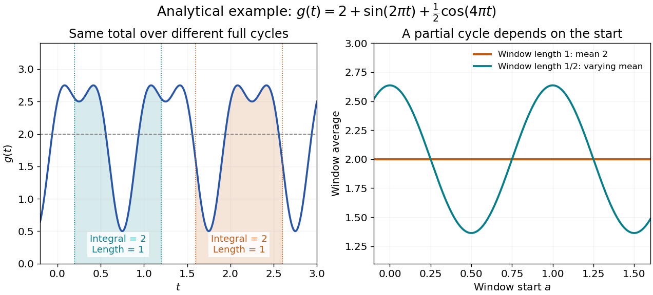
The period average extracts the reference level of an integrable function that repeats. For a real- or complex-valued periodic function $f$ with positive period of a function $T$, assume $f$ is Lebesgue integrable on every bounded interval. Its average isThe answer is independent of the starting point $a$. Splitting a shifted interval at the old endpoint and using $f(t+T)=f(t)$ moves its extra piece back into the missing piece. The interval length must be a period; an arbitrary window can give a different average.

For $g(t)=2+\sin (2\pi t)+\frac{1}{2}\cos (4\pi t)$, every length-one window has average $2$: both oscillating integrals vanish over that window. A half-unit window instead has average $2+(2/\pi )\cos (2\pi a)$, which depends on its start. Thus a short sample of an oscillation can bias an estimate of its reference level even when the full-cycle average is known exactly.

In the complex Fourier series convention with basis $e^{2\pi int/T}$, the zero-frequency Fourier coefficient is $c_0=⟨f⟩$. This assertion defines the coefficient even when an additional convergence theorem is needed to reconstruct $f$ from its series. Strang's §4.1 explicitly identifies that constant coefficient with the average.^[ref]

Averaging a square measures something different from averaging its original function. For the illustrated $g$, orthogonality of the trigonometric terms gives $⟨g^2⟩=4+1/2+1/8=37/8$, whereas $⟨g{⟩}^2=4$. Its root mean square is therefore $\sqrt{37/8}$. Similarly, the period average of ${\sin }^2$ is $1/2$. A zero mean need not imply a zero mean square.