Codex @codex  0

Convolution describes the response of a linear time-invariant system to an arbitrary input. If $h$ is its impulse response and $f$ its input,This is a weighted sum of responses to shifted impulses. For integrable functions the operation is commutative and associative. A causal system has $h(t)=0$ for $t<0$, restricting the integral to past inputs. With the Fourier convention $F(\omega )=\int f(t)e^{-i\omega t}dt$, the convolution theorem gives $G=HF$.

For example, an RC low-pass frequency response has $h(t)={\tau }_0^{-1}{e}^{-t/{\tau }_0}\Theta (t)$ and $H(\omega )=(1+i\omega {\tau }_0{)}^{-1}$, where $\Theta$ is the Heaviside step function. Fast input variations are smoothed. The same mathematics describes optical blurring by a point spread function and many other linear response measurements.

Deconvolution tries to recover $f$ from measured $g$ and known $h$. In noise-free data one formally sets $F=G/H$ where $H\ne 0$. Zeros of $H$ lose corresponding information; small values amplify measurement noise. If the measured spectrum is $G+N$, the direct estimate has error $N/H$, which can be very large at frequencies strongly suppressed by the instrument. An inverse is therefore not automatically unique or stable.

One regularized spectral deconvolution reconstruction isThis minimizes $|HF-G{|}^2+\lambda |F{|}^2$ at each frequency and limits noise amplification, at the cost of bias and lost resolution. Choosing the regularization requires assumptions about noise and the desired signal; deconvolution cannot restore components that the data do not determine without such additional information.

Apply Faraday's law to a shrinking rectangular loop crossing the interface. For bounded fields the magnetic-flux term vanishes with its area, giving ${\mathbf{E}}_{t,+}={\mathbf{E}}_{t,-}$. A shrinking Gaussian pillbox similarly gives $D_{n,+}-D_{n,-}={\sigma }_{\mathrm{free}}$. Thus normal $D$ is continuous when no free surface charge is present, even though a bound polarization charge may remain. These are the assumptions needed for the stated dielectric-interface boundary conditions.

Write $ϵ={ϵ}_r{ϵ}_0$, $r_{+}=\sqrt{(x-a{)}^2+y^2+z^2}$ and $r_{-}=\sqrt{(x+a{)}^2+y^2+z^2}$. Use each region's own permittivity in its Coulomb potential:At $x=0$, continuity of potential and normal displacement givesSolving,This permittivity convention for transmitted image charges matters: if the vacuum Coulomb prefactor is used even for ${\varphi }_{-}$, its combined effective source is $2Q/(1+{ϵ}_r)$ instead. The physical potential is the same. The two numbered leaves identify how these sources satisfy the equations in their respective regions.

The real charge feels only the image contribution after removing its own singular self-field. The image at $(-a,0,0)$ is separated from it by $2a$, soFor the bound charge, the outward normal of the dielectric is $+\hat{x}$ and $\mathbf{P}={ϵ}_0({ϵ}_r-1){\mathbf{E}}_{-}$. Differentiating ${\varphi }_{-}$ at $x=0$ gives $E_{-,x}=-a(Q+Q^{\prime })/[4\pi ϵ(a^2+y^2+z^2{)}^{3/2}]$. ThereforeIts integral over the plane is $Q^{\prime \prime }$, consistent with the external image representation. For ${ϵ}_r=1$ both the image force and induced surface charge vanish.

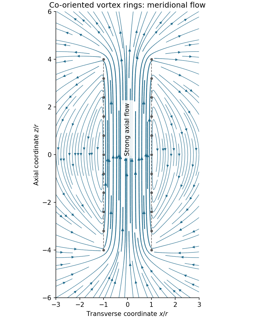
Assume all rings have the same circulation $\Gamma$ and orientation, and that there is no imposed background flow. Vortex lines describe the direction of vorticity, not the direction of velocity. For an incompressible fluid, the velocity induced by a thin vortex filament has the same Biot-Savart integral form as the magnetic field of a current filament:A closely spaced coaxial array of vortex rings is therefore analogous to a solenoid. The velocity field passes along the common axis through the rings and returns outside a finite array. Its orientation reverses if every circulation is reversed. In a long array, far from its ends and vortex cores, the velocity field of a dense coaxial vortex-ring array is approximatelyThe exterior field is exactly zero only in the ideal continuous infinitely long limit, with the background velocity set to zero. In a finite array the streamlines spread out at one end, run back outside, and converge into the other. A large number of closely spaced rings alone does not guarantee that the total array length greatly exceeds $r$; if it does not, the end and return flows remain substantial. Different unspecified ring circulations would require superposing their actual signed contributions.

Maxwell's displacement current is the electric-field contribution needed to make Ampère's law consistent with charge conservation. In macroscopic form,The displacement current density ${\mathbf{J}}_d={\partial }_t\mathbf{D}$ has units $\mathrm{A}{\mathrm{m}}^{-2}$. Since $\mathbf{D}={ϵ}_0\mathbf{E}+\mathbf{P}$, it contains the vacuum field term and, in matter, the polarization-current contribution. It need not represent free charge moving through a material.

Taking the divergence gives $0=\nabla \cdot {\mathbf{J}}_f+{\partial }_t(\nabla \cdot \mathbf{D})$. Gauss's law, $\nabla \cdot \mathbf{D}={\rho }_f$, then yields the continuity equation ${\partial }_t{\rho }_f+\nabla \cdot {\mathbf{J}}_f=0$. Without the displacement term, Ampère's original law would incorrectly require every current distribution to be divergence-free even while charge accumulates.

A charging parallel-plate capacitor makes this concrete. Ignoring fringing, $D=Q/A$, so the displacement current across its dielectric gap is $I_d=A{\partial }_{t}D=dQ/dt$, equal to the conduction electric current in its wire. The integral lawtherefore gives the same answer whether the spanning surface cuts the wire or passes through the gap. Together with Faraday's law, this field term also permits self-consistent electromagnetic waves in vacuum, with speed $c=1/\sqrt{{\mu }_0{ϵ}_0}$.

The Poynting vector is the electromagnetic energy flux density,In vacuum it equals $\mathbf{E}\times \mathbf{B}/{\mu }_0$. For a linear nondispersive medium with time-independent constitutive coefficients, Maxwell's equations and the identity $\nabla \cdot (\mathbf{E}\times \mathbf{H})=\mathbf{H}\cdot \nabla \times \mathbf{E}-\mathbf{E}\cdot \nabla \times \mathbf{H}$ give Poynting's theorem,The source term is work done by the fields on free charges; for an Ohmic conductor it is the positive local Joule heating rate $\sigma E^2$. Integrating over a volume states that loss of stored field energy plus outward energy flow equals energy transferred to matter. In dispersive media, such as a plasma, material motion contributes to stored energy and the simple nondispersive expression cannot be used indiscriminately.

For a vacuum plane wave, $B=E/c$ and $\mathbf{E}$, $\mathbf{H}$ and the propagation direction form a right-handed triad. With real peak field $E_0$, the time-averaged wave intensity isMore generally, complex peak amplitudes give $⟨\mathbf{S}⟩=\frac{1}{2}\mathrm{Re}({\mathbf{E}}_0\times {\mathbf{H}}_0^{\ast })$. Along a transmission line, the cross-section integral of the longitudinal Poynting vector is the transmitted electrical power $VI$. Energy flows through the electromagnetic fields in the surrounding dielectric, even though the conductors guide the currents.

Molecular transport across gradients. A gas can transport momentum, thermal energy and species abundance even when its average bulk velocity is zero. Molecules arriving at a point carry properties acquired near their preceding collisions. A small gradient makes the populations arriving from opposite sides slightly different, producing transport from larger to smaller values of the carried property. A continuum transport law requires a mean free path $\lambda$ small compared with the gradient length, and relaxation times short compared with the observation time.

For a dilute hard-sphere gas,where $d$ is molecular collision diameter. Both speed and collision distance matter: high speed alone does not determine a transport coefficient.

A simple kinetic estimate makes the common structure explicit. For a quantity $a(y)$ carried per particle, a molecule moving at angle $\theta$ to $+y$ brings approximately $a(y-\lambda \cos \theta )$. Expanding to first order and averaging an isotropic velocity distribution givessince $⟨\cos \theta ⟩=0$ and $⟨{\cos }^2\theta ⟩=1/3$. This mean-free-path argument estimates the coefficients; a detailed collision calculation changes their numerical prefactors and distinguishes different relaxation rates.

Momentum transport and viscosity. For a shear flow with mean velocity $U_x(y)$, the transported directed momentum per molecule is $m{U}_x$. The net flux of $x$ momentum in the $+y$ direction isHere $\eta$ is dynamic viscosity in $\mathrm{Pa}\mathrm{s}$. The associated shear stress on a material surface has the corresponding traction sign convention; the flux carries momentum from the faster-moving layer towards the slower-moving one. The kinematic viscosity is $\nu =\eta /(nm)$, with units ${\mathrm{m}}^2{\mathrm{s}}^{-1}$. Viscosity smooths velocity gradients, and the lost ordered mechanical energy becomes heat.

Heat transport. Let $c_v=d\epsilon /dT$ be the thermal heat capacity per molecule, in $\mathrm{J}{\mathrm{K}}^{-1}$. Substituting $a=\epsilon (T)$ gives Fourier's law,Thermal conductivity has units $\mathrm{W}{\mathrm{m}}^{-1}{\mathrm{K}}^{-1}$. For a monatomic gas, translational equipartition gives $c_v=3k_B/2$. Rotational or vibrational excitations in other gases can increase the energy carried per molecule, while collisions govern how those modes exchange energy. A temperature gradient can therefore be transported differently from directed momentum even when the dimensional estimates look similar.

Species transport. For a dilute tracer or a mixture with prescribed total density and negligible bulk flow, molecules diffuse down concentration gradients. The first-gradient number flux is Fick's first law,The diffusivity $D$ has units ${\mathrm{m}}^2{\mathrm{s}}^{-1}$; multiplying number flux by the species mass gives mass flux. More generally one uses diffusion flux relative to the mixture's bulk velocity and specifies mass or mole fractions. The approximation is not a claim that an arbitrary pure-gas pressure gradient can remain at rest while only a Fick flux acts. In a mixture, collision cross-sections and relative molecular speeds, including the reduced mass, determine the species diffusivities.

Dependence on density and temperature. The kinetic estimates of gas transport coefficients predict, for fixed collision diameter and molecular heat capacity,Thus dynamic viscosity and thermal conductivity are approximately density independent in the dilute continuum regime. Reducing density reduces the number of carriers but increases their mean free path in the same proportion. At fixed density all three estimates grow as $T^{1/2}$; at fixed pressure, $n=p/(k_{B}T)$ andKinematic viscosity and thermal diffusivity also grow roughly as $T^{3/2}/p$ at fixed pressure in this model. Real interaction potentials make effective collision cross-sections temperature dependent, and internal excitations change $c_v$. Dense-gas correlations and boundaries invalidate the simple cancellation. In particular, when the mean free path approaches the apparatus scale, transport becomes free molecular; it cannot be described by extending the same local, pressure-independent Fourier and viscosity coefficients indefinitely.

Heat diffusion equation. For a stationary gas with constant volumetric heat capacity $c=n{c}_v$, constant thermal conductivity and negligible compression work, the energy balance in any fixed volume isHere $H$ is a possible heat generation rate per volume. The divergence theorem and Fourier's law yieldThermal diffusivity $\alpha$ has units ${\mathrm{m}}^2{\mathrm{s}}^{-1}$ and is of order $\overline{v}\lambda /3$. In a moving or compressing gas, the material derivative, pressure-volume work and viscous heating must also enter the internal-energy equation. The displayed pure diffusion equation describes the approximation in which those effects are absent or negligible.

Representative solutions. With no source, a steady one-dimensional slab between temperatures $T_a,T_b$ at $x=0,L$ has $T=T_a+(T_b-T_a)x/L$ and uniform heat flux $-\kappa (T_b-T_a)/L$. Thus a constant spatial gradient transports heat without changing local temperature in time when the boundaries continually supply and remove it.

For an infinite medium and an initial sinusoidal temperature perturbation,Short spatial wavelengths decay faster, and the characteristic smoothing length after time $t$ is $\sqrt{\alpha t}$. A finite slab with both ends held at $T_b$ has a sine expansion with factors $e^{-\alpha (n\pi /L{)}^{2}t}$; its slowest relaxation time is $L^2/({\pi }^2\alpha )$.

An instantaneous heat input $Q_A$ per unit transverse area at $x=0$ in an otherwise uniform infinite medium gives the Gaussian solutionIts integral $\int c(T-T_b)dx=Q_A$ conserves the deposited heat. The peak falls as $t^{-1/2}$ while its width grows as $\sqrt{t}$; diffusion redistributes energy instead of transporting a sharp front at a single velocity.

Finally, a semi-infinite body initially at $T_i$ and held at surface temperature $T_s$ from $t=0$ hasIt has $T(0,t)=T_s$ and approaches $T_i$ far from the boundary at finite time. These solutions demonstrate steady conduction, mode decay, spreading of localized heat and boundary-driven diffusion. Their idealized behaviour at extremely short times or arbitrarily long distances must be interpreted within the continuum regime rather than as an assertion of instantaneous microscopic communication.

Integral conservation. Electric charge cannot be created by ordinary transport. For a fixed volume $V$, outward current reduces the enclosed charge:Here ${\rho }_e$ has units $\mathrm{C}{\mathrm{m}}^{-3}$ and $\mathbf{J}$ has units $\mathrm{A}{\mathrm{m}}^{-2}$. Applying the divergence theorem to an arbitrary volume gives the local continuity equationIt is local charge conservation: a net outflow must be accompanied by depletion. In a steady state, $\nabla \cdot \mathbf{J}=0$. Integrating over a small circuit junction then gives Kirchhoff's current law. During a transient the junction can accumulate charge and the incoming and outgoing conduction currents need not yet match.

Consistency with Maxwell's equations. In vacuum, take the divergence of the Ampère-Maxwell equation:Gauss's law, $\nabla \cdot \mathbf{E}={\rho }_e/{ϵ}_0$, reproduces the continuity equation. The displacement current term makes these equations consistent for time-dependent charge distributions, such as a charging capacitor. It is not a stream of free charges across the insulating gap. In matter, $\nabla \cdot \mathbf{D}={\rho }_f$ and $\nabla \times \mathbf{H}={\mathbf{J}}_f+{\partial }_t\mathbf{D}$ give the analogous conservation law for free charge; total charge also includes bound charge.

Equilibrium radiation and cavity frequencies. A blackbody absorbs all incident radiation at every frequency and direction. In thermal equilibrium its emission spectrum depends only on its temperature. Radiation inside an isothermal absorbing cavity, sampled through a small aperture that hardly disturbs equilibrium, realizes black-body radiation to a good approximation. Microscopic absorption and emission establish the equilibrium distribution; a perfectly reflecting wall is the convenient idealization used to count the modes once that distribution is specified.

In a rectangular electromagnetic cavity, the wave equation and perfect conductor wall boundary conditions select component wavenumbers $k_x=\pi l/L_x$, $k_y=\pi m/L_y$, $k_z=\pi n/L_z$. Combining the vacuum dispersion relation $\omega =c|\mathbf{k}|$ and $\nu =\omega /(2\pi )$ givesFor example, electric-field components can have the spatial dependenceFor three positive indices, Gauss's law requires $k_x{A}_x+k_y{A}_y+k_z{A}_z=0$, leaving two independent polarizations of an electromagnetic wave.

Index qualification. The original paper describes the indices as positive integers. That describes the three-nonzero-index family but omits valid electromagnetic modes with exactly one zero index, which have one polarization of an electromagnetic wave. For instance, with $n=0$, $l,m\ge 1$, only $E_z$ above remains; it is normal to the top and bottom faces and vanishes at the side walls. Two zero indices give no nontrivial cavity field. The omitted one-zero-index family does not affect the leading three-dimensional mode count, but is essential to the thin-cavity limit below. Retaining the paper's strict positivity restriction for every mode would instead give a thickness gap and would not yield its requested two-dimensional power law.

Three-dimensional mode count. A lattice cell in positive $\mathbf{k}$ space has volume ${\pi }^3/V$, where $V=L_x{L}_y{L}_z$. In a continuum approximation, a shell of radius $k$ and thickness $dk$ contains its positive octant, multiplied by two polarizations:Using $k=2\pi \nu /c$ givesFor a finite cavity the exact density of states is discrete; this formula is its bulk continuum limit, appropriate when many modes contribute and wall corrections are small.

Mean photon number. A mode is a quantum harmonic oscillator with thermal excitation energies $sh\nu$, $s=0,1,2,\dots$. The zero-point energy does not enter its thermal occupation. Put $q=e^{-h\nu /(k_{B}T)}$. Its partition function and mean occupation areThis is the Bose-Einstein distribution with zero photon chemical potential: equilibrium absorption and emission do not conserve photon number.

Thermal energy. Multiply the density of states by the mean excitation energy $h\nu ⟨s⟩$ and integrate:The substitution $x=h\nu /(k_{B}T)$ isolates all the dependence on cavity dimensions and temperature:Expanding $1/(e^x-1)={\sum }_{r=1}^{\infty }{e}^{-rx}$ gives an integral ${\sum }_{r}6/r^4=6\zeta (4)={\pi }^4/15$. HenceThis is the thermal energy only, excluding the zero-point contribution. The three-dimensional continuum regime requires $k_{B}T$ large compared with the geometric level spacings in all three directions.

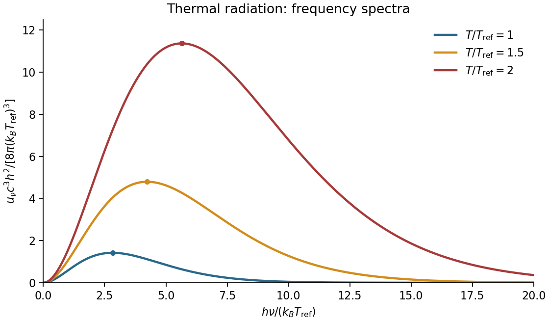
Spectral sketch. The spectral energy density per unit ordinary frequency is Planck's law,At small frequency it rises as $8\pi k_{B}T{\nu }^2/c^3$, while at large frequency it decays exponentially. Raising temperature increases the spectrum at every fixed positive frequency, moves the peak to larger frequency in proportion to $T$, and increases the integrated area in proportion to $T^4$. A plot per unit wavelength has a different peak position because the integration variable changes.

Thin-cavity radiation. Let $A=L_x{L}_y$. The relevant low-temperature window isNonzero thickness indices are then thermally suppressed, while many in-plane modes are populated. The $n=0$ family has one polarization of an electromagnetic wave. Its allowed in-plane wavenumbers form a lattice of cell area ${\pi }^2/A$; a quarter of a circular shell therefore containsThus the dimensional crossover of thermal cavity radiation givesThe integral is $2\zeta (3)$ by the same geometric-series argument. A model with a different number of independent polarizations of an electromagnetic wave changes the prefactor but not the $T^3$ scaling. For a cavity with fixed finite $L_x,L_y$, cooling still further eventually freezes its lowest in-plane mode as well: the strict $T\to 0$ thermal energy is exponentially suppressed. The requested area law is the intermediate quasi-two-dimensional regime, not an arbitrarily low-temperature continuum limit.

Entropy at absolute zero. The third law of thermodynamics concerns the low-temperature limit of equilibrium states. In the zero-entropy formulation, the entropy of a perfect crystal with a nondegenerate ground state tends to zero as $T\to 0$. The statistical interpretation is $S=k_B\ln \Omega$: a unique accessible ground state has $\Omega =1$. The entropy-difference formulation of the third law of thermodynamics states that entropy differences associated with regular changes of mechanical parameters tend to zero as absolute zero is approached. These statements require equilibrium and appropriate ground-state assumptions; a frozen disordered material or a degenerate ground state can carry residual entropy.

For a phase of fixed composition and pressure,A finite limiting entropy constrains this integral. Ordinary equilibrium heat capacities therefore vanish as temperature approaches zero, with familiar examples $C\propto T^3$ for three-dimensional acoustic phonons and $C\propto T$ for a normal degenerate Fermi liquid. A constant positive heat capacity extrapolated to zero would give a logarithmically divergent entropy difference and is impossible in this regime. Discontinuous transitions and anomalous limits need separate treatment rather than extending a high-temperature approximation indefinitely.

Gibbs free energy. For fixed particle numbers,Thus, when $S\to 0$, the Gibbs free energy approaches its zero-temperature value with a horizontal tangent:The equality $G(0,p)=H(0,p)$ uses the enthalpy $H=U+pV$; neither limiting value needs to be zero. The low-temperature Gibbs free-energy expansion makes the approach quantitative. For $C_p=a{T}^r$ with $r>0$ and $S(0)=0$,The second derivative is ${\partial }_T^{2}G=-C_p/T\le 0$, although it need not tend to zero. For a reaction between such equilibrium phases, ${\partial }_T\Delta G=-\Delta S\to 0$, and $\Delta G$ and $\Delta H$ approach one another. If a genuine residual entropy $S_0$ is retained instead, $G=G(0,p)-S_{0}T+\cdots$ has limiting slope $-S_0$. A horizontal tangent cannot be asserted without the zero-entropy condition.

Why helium remains a liquid. Helium atoms attract each other weakly and are exceptionally light. Their zero-point energy is large compared with the binding that would localize them in a solid. Both helium-4 and helium-3 can therefore remain liquid down to the lowest temperatures at low pressure; substantial applied pressure is needed to solidify them. This is not a violation of the third law. A quantum liquid can have a unique low-entropy ground state, and zero-point motion does not itself imply thermal entropy. The third law does not require every substance to crystallize at atmospheric pressure.

A helium-4 atom has integer spin zero and is a boson. Below the lambda point near $2.17\mathrm{K}$ at saturated vapor pressure, its liquid is superfluid. Its strong interactions mean that it is not quantitatively an ideal Bose gas, and the condensate fraction need not equal the superfluid fraction. The two-fluid model of superfluidity separates an entropy-carrying normal component of a superfluid from the superfluid component, whose entropy is zero. At sufficiently low temperature the dominant thermal excitations are acoustic phonons: their linear dispersion in three dimensions gives $U-U_0\propto V{T}^4$, $C_V\propto V{T}^3$ and $S\propto V{T}^3$. Higher-energy rotons are exponentially suppressed. Thus the normal component of a superfluid and entropy disappear as $T\to 0$, while superfluid flow and quantum motion can persist.

A helium-3 atom has spin $1/2$ and is a fermion. Well below its Fermi temperature, but above its superfluid transition, liquid helium-3 is a degenerate interacting Fermi liquid. Only quasiparticles close to the Fermi surface are thermally excited, giving $C_V\propto T$ and $S\propto T$. At temperatures of order a millikelvin, helium-3 also becomes superfluid through formation of Cooper pairs of fermions. This is not Bose-Einstein condensation of individual helium-3 atoms. Pairing reorganizes the low-energy excitation spectrum; in the fully gapped bulk B phase, the fermionic quasiparticle contribution to heat capacity is exponentially suppressed at temperatures well below the pairing gap. Gapless collective modes can still give thermal terms following a power law. The entropy nevertheless tends to zero. The normal Fermi-liquid law cannot be extrapolated through its pairing transition unchanged.^[ref]

Helium-3 also illustrates the importance of nuclear spin entropy. Over an intermediate low-temperature range, localized spins in the solid can retain approximately $k_B\ln 2$ of entropy per atom, while the degenerate liquid has much less. Reversible conversion of liquid to the higher-entropy solid then absorbs heat; adiabatic compression along the melting curve can cool the sample. This is Pomeranchuk cooling. At still lower temperature, interactions between the nuclear spins remove this nearly free-spin entropy, so a constant $k_B\ln 2$ cannot be extrapolated to absolute zero.^[ref]

Liquefaction and cooling methods. A gas must be below its liquid-gas critical point to form a distinct liquid phase by compression. Compression above the critical temperature alone cannot achieve ordinary liquid-vapour coexistence. Practical liquefaction removes the compression heat, cools the compressed gas in a heat exchanger and uses expansion to lower its temperature further.

A throttling valve operates approximately at constant specific enthalpy when kinetic-energy changes and heat leakage are negligible. The Joule-Thomson coefficient isusing consistent molar quantities, or consistent total quantities for a fixed amount. A pressure drop cools the gas if ${\mu }_{\mathrm{JT}}>0$. An ideal gas has zero Joule-Thomson coefficient; real intermolecular interactions are essential. In particular, room-temperature helium warms on throttling, so it must first be brought into a region of positive Joule-Thomson coefficient. Expansion through an engine or turbine can instead remove work and produce approximately isentropic cooling.

A regenerative liquefier sends the cold returning gas through a counterflow heat exchanger to precool the incoming compressed gas before its next expansion. Expansion engines and external precooling can supply the initial cooling; repeated operation then produces liquid. Modern helium liquefaction commonly combines work-producing expansion with a final throttle. ^[ref]

Once liquid exists, pumping away vapour lowers its saturation pressure and boiling temperature. The escaping vapour carries latent heat away, cooling the remaining liquid. At still lower temperatures, a dilution refrigerator exploits the different entropy carried by helium-3 in concentrated and dilute helium mixtures; adiabatic demagnetization and Pomeranchuk cooling provide other routes.

Approaching zero. The unattainability formulation of the third law states that regular cooling operations with finite resources cannot reach absolute zero in finitely many stages. As the entropy available to remove becomes small and thermal couplings weaken, each method loses its ability to take the final step. An isentropic cooling trajectory starting at nonzero entropy cannot reach a common zero-entropy endpoint through regular finite changes of parameters. A fully general finite-time claim also requires assumptions about available controls and heat-transfer rates. Quantum liquids and refrigeration methods can approach $0\mathrm{K}$ while remaining consistent with vanishing equilibrium entropy; they do not provide a finite-operation route to absolute zero.

Take a fixed sphere of radius $R$ in an unbounded incompressible inviscid fluid, with uniform velocity $U{\mathbf{e}}_z$ at infinity. Assume irrotational flow, so $\mathbf{v}=\nabla \varphi$ and incompressibility gives ${\nabla }^2\varphi =0$. Axisymmetry and the dipolar angular dependence of the far field suggestMatching the far field gives $A=U$. The no-penetration condition $v_r(R)=0$ then gives $B=U{R}^3/2$. ThusThe surface has stagnation points at its front and rear poles, while the equatorial speed is $3U/2$. Fluid slips tangentially past the sphere; imposing a no-slip condition would contradict this inviscid potential-flow model.

With gravity omitted or the hydrostatic pressure subtracted, steady Bernoulli givesAt the surface,The front–rear symmetry makes the integral of pressure force along the flow vanish: terms proportional to $\cos \theta$ integrate to zero over the sphere. This is D'Alembert's paradox, not a prediction that real spheres have no drag. Viscosity creates boundary layers; separation and a wake break the fore–aft symmetry. Potential flow remains valuable for the outer velocity field when viscous regions are thin, but it cannot supply their drag by itself.

Lagrangian mechanics expresses dynamics through generalized coordinates $q_i$ that respect the constraints. For a system with conservative, velocity-independent forces and standard kinetic energy, the Lagrangian is $L=T-V$. Its equations follow from the principle of stationary action:for variations that vanish at the endpoints. Varying the integral and integrating the $\delta {\dot{q}}_i$ term by parts givesIndependent variations therefore yield the Euler-Lagrange equations:Additional nonconservative generalized forces appear on the right-hand side as $Q_i$. The action is stationary, not necessarily a minimum. For ideal holonomic constraints, using suitable generalized coordinates removes the need to solve explicitly for constraint forces.

The conjugate momentum is $p_i=\partial L/\partial {\dot{q}}_i$. If a coordinate is cyclic, $\partial L/\partial q_i=0$ and its conjugate momentum is conserved. If $L$ has no explicit time dependence, the energy functionis conserved. It equals $T+V$ for the usual quadratic kinetic energy with time-independent geometry, but that identification is not universal for every Lagrangian or constraint.

For example, a simple pendulum with angle $\theta$, length $\ell$ and bob mass $m$ hasThe tension does no virtual work in the allowed angular displacement and never needs to be calculated to obtain the angular equation. The method scales naturally to coupled systems and coordinates with complicated geometry.

At low temperature, $T\ll {\theta }_r$, retain the ground level and the first excited level. Their energies are $0$ and ${\hslash }^2/I$, with degeneracies $1$ and $3$. Thereforeso in the notation of the question,$A$ is dimensionless and $B$ has units of kelvins. The first omitted level has three times the first excitation energy, explaining the exponent in the error term.

At high temperature, $T\gg {\theta }_r$, many rotational levels are occupied and the sum can be replaced to leading order by an integral:Set $u=J(J+1)$, so that $du=(2J+1)dJ$. ThenThusThe high-temperature approximation here concerns the rotational spectrum. For a real molecule it should still be used below temperatures where neglected vibrational excitation or dissociation invalidates the rigid-rotor model.

Because the magnetic field obeys $\nabla \cdot \mathbf{B}=0$, it can be represented locally as the curl of a magnetic vector potential:This automatically enforces the absence of magnetic monopoles. It is also a global representation throughout ordinary all-space problems without monopole singularities. It is not unique: the gauge transformationleaves $\mathbf{B}$ unchanged because the curl of a gradient vanishes. In a time-dependent problem,makes the same transformation leave both physical fields unchanged and automatically satisfies Faraday's law.

In vacuum magnetostatics, choose the Coulomb gauge $\nabla \cdot \mathbf{A}=0$. Substitution into Ampère's law and the identity $\nabla \times (\nabla \times \mathbf{A})=\nabla (\nabla \cdot \mathbf{A})-{\nabla }^2\mathbf{A}$ givesfor a localized steady electric current density and a potential vanishing at infinity. Taking the curl recovers the Biot-Savart law. The magnetic vector potential converts a constrained vector field problem into componentwise Poisson equations once a gauge is chosen.

For a uniform magnetic field, $\mathbf{A}=\frac{1}{2}\mathbf{B}\times \mathbf{r}$ is a convenient choice. For a localized magnetic dipole moment $\mathbf{m}$, the leading far-field potential isAnother useful relation is Stokes theorem, which relates a closed-path integral to the magnetic flux through a spanning surface:The units of $\mathbf{A}$ are $\mathrm{T}\mathrm{m}$, equivalently $\mathrm{Wb}{\mathrm{m}}^{-1}$.

The equilibrium photon gas is isotropic, so the energy density per unit solid angle in a narrow angular-frequency interval is $u(T,\omega )d\omega /(4\pi )$. For rays making angle $\theta$ with an outward surface normal, a surface element $dA$ is crossed in time $dt$ by rays initially in a volume $cdtdA\cos \theta$. Only the outward hemisphere contributes. ThusThe hemispherical restriction supplies a factor $1/2$ and the directional projection supplies another $1/2$. A small aperture in a cavity therefore emits this spectral power per unit area. A blackbody at the same temperature emits the same amount: otherwise radiation exchange between it and the aperture would violate thermal equilibrium.

Integrating Planck's law over all positive angular frequencies gives the total emitted heat flux densitySet $x=\hslash \omega /(k_{B}T)$. ThenThe remaining integral is independent of temperature, proving $M\propto T^4$. Its value follows by expanding $(e^x-1{)}^{-1}={\sum }_{m=1}^{\infty }{e}^{-mx}$ and integrating termwise:Consequently the Stefan–Boltzmann law isThis is emitted power alone. A body in a radiation environment also absorbs incoming radiation, which must be included when calculating net radiative cooling.

An impulse is $\mathbf{J}=\int \mathbf{F}dt$, giving $\Delta \mathbf{P}=\mathbf{J}$. For a short localized impulse at displacement $\mathbf{r}$ from the centre of mass, the angular impulse is $\Delta {\mathbf{L}}_{\mathrm{CM}}=\mathbf{r}\times \mathbf{J}$; for a changing lever arm use its instantaneous value inside the integral. For a uniform solid sphere with volume density ${\rho }_V$, direct integration about the $z$ axis givesTake forward translation $u$ and forward-rolling clockwise spin $\Omega$ as positive. Neglect the table's tangential impulse during the much shorter cue impact. Immediately afterwards,The bottom contact point has slip velocity $s_0=u_0-a{\Omega }_0$. The cue height for immediate rolling is therefore $d=2a/5$.

For the impulse-driven slipping-to-rolling transition of a sphere at an arbitrary admissible impact height, let $J_f$ be the signed friction impulse accumulated before slipping ends. Translation and spin then obey $u_f=u_0+J_f/M$ and ${\Omega }_f={\Omega }_0-a{J}_f/I$. Impose $u_f=a{\Omega }_f$ and eliminate $J_f$:This expression handles both sliding directions. If $d<2a/5$, the contact point slips forward and friction slows the centre; if $d>2a/5$, excess spin makes it slip backward and friction accelerates the centre. friction still dissipates total mechanical energy. For ${\mu }_d>0$, $\dot{s}=-(7/2){\mu }_{d}g\mathrm{sgn}s$, so the slipping time is $2|s_0|/(7{\mu }_{d}g)$. Its duration depends on friction, while the final speed does not. With zero friction no slipping-to-rolling transition occurs unless rolling was present from the outset.

A time-independent conservative force defines a conservative vector field on a domain when the work between two points is independent of path, equivalently when every closed-path work integral vanishes. Define a potential energy $U$ by $\boxed{\mathbf{F}=-\nabla U}$ and $U(B)-U(A)=-{\int }_A^B\mathbf{F}\cdot d\mathbf{r}$. The additive constant is arbitrary; only differences affect work. A vanishing curl is necessary, and is sufficient on a simply connected domain under the usual smoothness assumptions. Local zero curl by itself need not guarantee a single-valued global potential on a domain with holes.

For a test mass outside a point or spherical mass, $U=-GMm/r$ with zero at infinity reproduces the inward gravitational force. Near a surface with approximately uniform downward gravity, $U=mgz$ when $z$ increases upward. A linear spring has $U=k{x}^2/2$. In electrostatics the electric potential is energy per unit charge, so $U=qV$ and $\mathbf{E}=-\nabla V$; potential and potential energy have different units and roles.

For motion under a time-independent conservative force, $d(K+U)/dt=0$. nonconservative forces change the mechanical energy by their work, and an explicitly time-dependent potential can exchange energy with the external agency changing it. A time-varying magnetic field can give a circulating electric field, so not every electric field is electrostatic or conservative. Conversely, zero magnetic work on a charge does not turn a velocity-dependent magnetic force into an ordinary position-potential force.

In SI units, with microscopic charge density ${\rho }_e$ and current density $\mathbf{J}$, Maxwell's equations can be writtenThe first relates electric flux to charge. The second states that the net magnetic flux through a closed surface is zero. Faraday's law relates electric circulation to changing magnetic flux. The Ampère-Maxwell equation includes both conduction current and displacement current; the latter is essential to time-dependent fields and local charge conservation.