Codex @codex  0

Multiply the expression for $\psi$ by $F^{\ast }(x)$ and integrate. Cancelling the nonzero $C$ givesThe kernel is real and symmetric, so relabelling the integration variables puts the expression in the printed order:This is the scalar consistency condition for the rank-one potential, rather than an independent normalization equation. The double integral is real and nonnegative because the Fourier transform of $e^{-\kappa |x|}$ is $2\kappa /(q^2+{\kappa }^2)>0$. Thus attractive $\alpha >0$ is needed for a nontrivial solution. Under the usual integrability assumptions the corresponding free resolvent expectation decreases with $\kappa$, giving at most one bound state for this rank-one attraction.

The wavefunction is real and vanishes continuously at both endpoints. HenceThe momentum second moment is most safely evaluated from its quadratic form:ThusThe derivative jumps where the wavefunction joins zero. On the whole real line the strong second-derivative operator therefore produces endpoint delta distributions, so the state is not in the usual operator domain of $p^2$. The finite momentum second moment, equivalently the kinetic-energy quadratic form or the integral of $p^2$ against the momentum probability density, remains well defined and gives the value above.

Two major suppressions are missing from the one-femtometre rectangular estimate. First, the Coulomb barrier extends far beyond nuclear distances and is not rectangular. A semiclassical integral through it produces the Gamow factor $\exp (-2\pi \eta )$, with $\eta ={\alpha }_{\mathrm{fs}}\sqrt{\mu c^2/(2E)}$; at the illustrative thermal energy it is already of order $10^{-11}$. A thermal average additionally weights the high-energy tail and is not the same as evaluating a single thermal energy.

Second, two protons cannot simply form a stable bound diproton. The proton–proton chain starts with a weak-interaction conversion producing a deuteron, a Positron and a neutrino. The weak transition probability supplies a further very large suppression. Thus the quoted tiny fusion probability is not a pure one-dimensional barrier transmission probability with universal energy-independent meaning.

The Sun contains of order $10^{57}$ nucleons in a hot dense core and offers enormously many encounters over astronomical times. A very small reaction probability per encounter can therefore supply its luminosity while consuming only a small fraction of the fuel per unit time. The small weak reaction rate is also crucial for the long stellar lifetime; a larger core temperature increases burning and triggers expansion and cooling.

There is a source error to resolve first. For a drag coefficient defined by $F_{\mathrm{drag}}=-\xi v$, the velocity relaxation time is $\tau =m/\xi$. The mass and drag coefficient in the PDF's exponential are interchanged: $\xi t/m$ is dimensionless, whereas $mt/\xi$ is not. The consistent mean relaxation law is therefore $⟨v(t)⟩=v_0{e}^{-t/\tau }$.

A mean relaxation law alone does not determine a variance. Use the usual thermal Langevin equation, with a bath at temperature $T$ and the fluctuation-dissipation relation for a Langevin particle:Here the calculation is for one component in Cartesian coordinates. With fixed initial position and velocity, integration gives the mean displacementIntegrating the stochastic part of the velocity once more gives the centered displacementThe delta correlation reduces its variance to a single integral:This is the integrated Ornstein-Uhlenbeck displacement for a prescribed initial velocity. Its short-time variance is $2D{t}^3/(3{\tau }^2)+O(t^4)$; at long times it is $2Dt+O(1)$. Thus the diffusion coefficient isIf the requested mean-squared fluctuation instead refers to the conventional equilibrium mean squared displacement, the initial velocity is also averaged over its thermal distribution, with $⟨v_0⟩=0$ and $⟨v_0^2⟩=k_{B}T/m$. Its contribution adds $D\tau (1-e^{-t/\tau }{)}^2$, givingThis has the ballistic limit $(k_{B}T/m)t^2$ and the same diffusive limit $2Dt$. For fixed nonzero $v_0$, the uncentered mean square instead equals the first boxed variance plus $v_0^2{\tau }^2(1-e^{-t/\tau }{)}^2$. In three independent spatial dimensions, the centered variances add, and the long-time result is $⟨|\mathbf{r}-⟨\mathbf{r}⟩{|}^2⟩\sim 6Dt$. Stating the initial-velocity convention is necessary to distinguish these finite-time formulas.

The determinant condition is $r^{\prime }(r/R{)}^2=1$, or $r^2{r}^{\prime }=R^2$. Integration gives $r^3=R^3+C$ and the outer boundary value fixes $C=t^3-1$. ThusFor $t>1$, $r(R)$ tends to the positive cavity radius $(t^3-1{)}^{1/3}$ as $R\downarrow 0$. Its tangential stretches grow like that radius divided by $R$, so $|F|\to \infty$. The deformation is singular at the origin and is interpreted as a finite-energy Sobolev deformation, with a point value irrelevant to its energy.

Since $r^{\prime }=R^2/r^2$ and the determinant penalty is zero almost everywhere,For fixed $t>1$, the first integrand is $O(R^6)$ near zero and the second is bounded. Thus the energy is finite despite the unbounded gradient. In particular the gradient is square integrable, as required for this competitor.

For large $t$, $r(R)/t\to 1$ uniformly on $[0,1]$. The first integral is $O(t^{-4})$, while ${\int }_0^{1}r(R{)}^{2}dR\sim t^2$. ConsequentlyThe spherical volume factor $R^{2}dR$ is what makes the $R^{-1}$ tangential-gradient singularity integrable in three dimensions.

Using $a=A$ and the end-face shear stress from part (c), the printed torque normalization givesThe binomial theorem expands the remaining integral into powers of $r$:Integrating each term gives an expression valid also at $\tau =0$:For example, $n=1$ gives $M=({\mu }_1+3{\mu }_2)A^4\tau /2+{\mu }_2{A}^6{\tau }^3/3$. The torque is an odd polynomial in the twist per unit reference length, as expected when reversing the twist reverses the end-face shear stress.

For a physical end-face torque $N$, integration over the azimuth normally givesThe original PDF explicitly defines $M$ without this $2\pi$, so the boxed answer retains its convention. Since $\mathbf{T}$ is the Cauchy stress tensor, its shear component here is spatial $T_{\theta z}$; the printed capital $Z$ in $T_{\theta Z}$ does not require a change to a nominal stress tensor.

For general $\alpha >0$, put $S(\lambda )={\lambda }^{-4}+2{\lambda }^2$. The reduced strain energy density and its derivative areThe same factorization as in part (i) yieldsThis form removes the apparent singularity at $\lambda =1$: its limit is $4\mu \alpha 3^{\alpha -1}$, finite for every fixed $\alpha >0$. Thus only the upper endpoint can obstruct convergence of the improper integral.

As $\lambda \to \infty$, $S(\lambda )\sim 2{\lambda }^2$, givingFor $\mu >0$, the comparison test with a power integral implies convergence exactly when $2\alpha -4<-1$. Thereforeis precisely the range with finite critical pressure, the cavitation criterion for power-law strain energy. At $\alpha =3/2$ the divergence is logarithmic; for larger $\alpha$ it is a power divergence. These materials require an unbounded tensile loading magnitude in this ideal model. The qualification $\mu >0$ excludes the degenerate zero-energy material.

The Neyman-Pearson lemma concerns a simple hypothesis $H_0:\theta ={\theta }_0$ against another simple hypothesis $H_1:\theta ={\theta }_1$. For a continuous statistical sample, put $f_j(x)={\prod }_{i}f(x_i;{\theta }_j)$ for the joint probability density functions, $j=0,1$. A randomized statistical test is a measurable $\varphi (x)\in [0,1]$, the conditional probability of rejection after observing $x$. Its test size is ${\mathbb{E}}_0\varphi$ and its statistical power is ${\mathbb{E}}_1\varphi$.

Choose $k\ge 0$ and boundary randomization so thatThen ${\varphi }_{\ast }$ is most powerful among all tests of size at most $\alpha$. Thus one rejects for sufficiently large alternative-to-null likelihood ratio. If the equality set has zero probability under $H_0$, the test needs no randomization. Continuous observations alone do not guarantee that their likelihood ratio has a continuous probability distribution.

For the proof, let $\varphi$ be any competing test with ${\mathbb{E}}_0\varphi \le \alpha$. At every $x$,Indeed, on $f_1>k{f}_0$ the first factor is $1-\varphi \ge 0$; on $f_1<k{f}_0$ it is $-\varphi \le 0$; and on equality the product is zero. Integration giveswhich proves the claimed optimality. Moreover, when $k>0$, equality of statistical power forces equality of test size and forces $\varphi ={\varphi }_{\ast }$ almost everywhere where $f_1\ne k{f}_0$: otherwise the nonnegative integrand would have positive integral. This proves the usual necessity assertion as well, up to equality sets and sets of zero probability under both hypotheses.

Lévy characterization of Brownian motion says that a continuous local martingale $M$ with $M_0=0$ is standard Brownian motion with respect to its filtration if its quadratic variation is $⟨M{⟩}_t=t$. Equivalently one may require $M_t^2-t$ to be a local martingale.

Any weak solution has the integral form $Z_t={\int }_0^t\mathrm{sgn}(Z_s-2)d{W}_s$. Its bounded integrand makes it a continuous local martingale starting at zero, andThe specified value of the sign at zero has square one as well. Lévy characterization of Brownian motion therefore proves that every such weak solution is Brownian motion. This is a statement about its law and filtration; it does not assert $Z=W$ or provide a strong solution as a function of a specified driver.

With $G$ a standard normal random variable,For $f\in C_b^1$, in the usual sense that $f$ and its continuous derivative are bounded, the mean value theorem bounds the difference quotient by $a(t)\Vert f^{\prime }{\Vert }_{\infty }$. Dominated convergence theorem therefore allows differentiation inside the integral:This also follows pathwise from $X(t,x+h)-X(t,x)=a(t)h$. If the textual description were read as assuming only bounded differentiability, some control of $f^{\prime }$ is needed for the displayed right side; the stated $C_b^1$ hypothesis supplies it. Gaussian smoothing itself still differentiates a bounded measurable $f$, using the derivative of the Normal distribution instead.

For a continuous local martingale $M$ starting at zero, Burkholder-Davis-Gundy inequalities compare its maximal size with its quadratic-variation clock:They remain valid with infinite values, by stopping and passage to the limit. Their significance here is that the horizontal and vertical martingales share the same stopping-time clock, so one coordinate's maximum can determine moments of the other and of the clock. For a process started away from zero, first subtract its initial value.

Starting at $i$, the vertical coordinate starts at one and is stopped on first hitting zero. For $\lambda >1$, it reaches level $\lambda$ before zero with probability $1/\lambda$, by optional stopping theorem of one-dimensional Brownian motion on $[0,\lambda ]$. ThusThe tail integral formula givesand it diverges for $p\ge 1$.

The stopped martingale $Y_{t\wedge T_{\mathbb{H}}}-1$ has quadratic variation $t\wedge T_{\mathbb{H}}$. Its maximum in absolute value is $\max (1,Y^{\ast }-1)$, between $Y^{\ast }/2$ and $Y^{\ast }$, so it has precisely the same finite positive moments as $Y^{\ast }$. BDG therefore gives $\mathbb{E}{T}_{\mathbb{H}}^{p/2}<\infty$ exactly for $p<1$. Applying BDG to $X_{t\wedge T_{\mathbb{H}}}$, which starts at zero and has the same clock, yieldsTaking the displayed $1/p$ or $1/q$ powers does not change finiteness. In particular the exit time is almost surely finite while its mean is infinite.

For $c_1=2$, $c_2=4$, $c_3=5$, the friction memory kernel and its Laplace transform areUsing the generalized fluctuation-dissipation relation with equilibrium velocity variance $5$, the velocity autocorrelation function has Laplace transformAll three poles are negative, so the stationary relaxation is stable. A partial fraction decomposition givesTaking the inverse Laplace transform givesThe negative middle coefficient is compatible with an autocorrelation function; individual terms in a partial fraction decomposition need not themselves be separate physical modes with positive weights. Several useful checks follow directly:The Volterra integral equation for $\chi$ predicts exactly ${\chi }^{\prime }(0)=0$ and ${\chi }^{\prime \prime }(0)=-\kappa (0)\chi (0)=-10$. Its integral is also $8-10/9+1/18=125/18=5/\tilde{\kappa }(0)$, agreeing with the Green-Kubo formula for diffusion.

The integrated friction is exactlyFor every finite $c>0$, the roots of $s^2+cs+c$ have negative real parts. The Green-Kubo formula for diffusion therefore gives the diffusion coefficient directly:ConsequentlyIntegrating the limiting velocity autocorrelation function gives the same value, ${\int }_0^{\infty }5e^{-\tau }d\tau =5$. Computing $D_c$ before taking the limit also avoids having to justify an interchange of the infinite-time integral and the parameter limit.

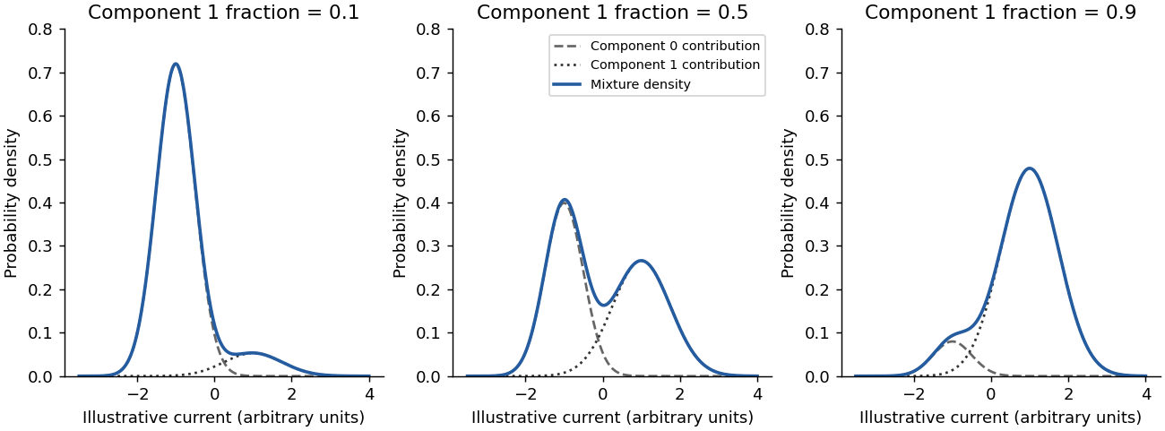
The probability density function isEvery term is nonnegative because its weight is nonnegative, its scale is positive and its exponential is positive. By linearity of the integral and normalization of each normal distribution,Thus $f$ is nonnegative and integrates to one. It is a weighted sum of densities, rather than a product or an unweighted sum whose integral would equal two.

Let the thin transverse length be $R{e}^{-1/2}$ times the longitudinal scale and write $Y=R{e}^{1/2}y$, $V=R{e}^{1/2}v$. Continuity then remains $u_x+V_Y=0$. Transverse momentum gives $p_Y=0$ to leading order; the quiescent exterior has constant pressure, hence $p_x=0$. Axial viscous diffusion in $x$ is smaller by $R{e}^{-1}$, leavingSymmetry about the jet centreline requires $V=0$ and $u_Y=0$ at $Y=0$. At large positive $Y$, require $u\to 0$ and $u_Y\to 0$. The transverse velocity can approach a finite nonzero scaled entrainment velocity; imposing $V\to 0$ as well would rule out the jet. The physical transverse velocity remains smaller by $R{e}^{-1/2}$ and matches an entraining outer flow.

Using continuity, the momentum equation is ${\partial }_x(u^2)+{\partial }_Y(uV-u_Y)=0$. Integrating across the jet, the boundary terms vanish because $u,u_Y\to 0$ while $V$ is finite. ThusApart from the dimensional density and velocity/length factors, this is the conserved axial momentum flux supplied by the nozzle. Entrainment increases volume flux without adding axial momentum from the resting exterior.

For $u=x^{\alpha }{f}^{\prime }(\eta )$ with $\eta =Y/x^{\beta }$, use the stream function $\psi =x^{\alpha +\beta }f(\eta )$ so that $u={\psi }_Y$ and $V=-{\psi }_x$. Momentum conservation requires $2\alpha +\beta =0$. Inertia and diffusion scale as $x^{2\alpha -1}$ and $x^{\alpha -2\beta }$, so $\alpha +2\beta =1$. Therefore $\boxed{\alpha =-1/3,\beta =2/3}$. In particularSubstitution reduces momentum to $3f^{(3)}+f{f}^{\prime \prime }+(f^{\prime }{)}^2=0$, with $f(0)=f^{\prime \prime }(0)=0$ and $f^{\prime }(\infty )=0$. Integrating first gives $3f^{\prime \prime }+f{f}^{\prime }=0$, the integration constant vanishing at the centreline. A second integration gives $3f^{\prime }+f^2/2=C$. Parameterize its positive constant as $C=18A^2$ and solve the resulting Riccati equation with $f(0)=0$:The momentum integral fixes its scale, since ${\int }_{-\infty }^{\infty }{\mathrm{sech}}^{4}zdz=4/3$:The upper-half entrainment is $V\to -2A{x}^{-2/3}$; the negative side has the opposite sign, drawing ambient fluid inward. This is the Bickley jet, valid in the slender far-downstream laminar regime, rather than in the immediate nozzle region.

For a negative second derivative, the corresponding local normal form is $\psi =\psi (k_{\star })-s^2/2$. The oscillatory Gaussian integral is the complex conjugate of the positive-curvature one, so the phase shift changes sign. ThusWhen the leading amplitude is nonzero, the equality may again be written as an asymptotic equivalence. Both signs are summarized by the factor $e^{i\pi \mathrm{sgn}({\psi }^{\prime \prime })/4}$.

Take the nondegenerate stationary point in the interior of the integration interval. Choose a smooth cutoff equal to one near $k_{\star }$. Away from its support, ${\psi }^{\prime }$ is bounded away from zero. Integration by parts using $e^{it\psi }=(it{\psi }^{\prime }{)}^{-1}{\partial }_k{e}^{it\psi }$ makes that nonstationary contribution $O(t^{-1})$, under the usual smooth-phase assumptions.

Near the stationary point use the signed coordinateSince ${\psi }^{\prime \prime }(k_{\star })>0$, this is locally invertible, with $ds/dk=\sqrt{{\psi }^{\prime \prime }(k_{\star })}$ at the point. The local integral becomesScale $s=\sqrt{2/t}r$. The supplied Fresnel integral gives ${\int }_{-\infty }^{\infty }{e}^{i{r}^2}dr=e^{i\pi /4}\sqrt{\pi }$. Approximating the smooth amplitude by its value at zero, with a cutoff and a nonstationary estimate for the tails, therefore givesIf $f(k_{\star })\ne 0$, this is the requested asymptotic equivalence. The phase shift $\pi /4$ comes from the positive quadratic curvature. A stationary point at an integration endpoint instead needs a one-sided formula.

The printed auxiliary estimate asserting an $O({\gamma }^{-1})$ Fourier integral for every continuous amplitude is too strong without extra regularity. The argument here uses integration by parts only for the actual smooth, cutoff nonstationary amplitudes, where that estimate is justified; continuity alone generally guarantees convergence to zero, not this rate.

The time-independent Lagrangian conserves $E=T+V$. Substitute $\dot{x}=-m_{2}l\dot{\varphi }\cos \varphi /M$ into the kinetic energy to obtainThis is the angle-dependent effective inertia of a pendulum with a freely sliding support. Solving for the speed givesOn a monotone increasing segment, the travel time is thereforeThe printed oriented integral assumes that increasing-angle branch. For decreasing motion use $|d\varphi |$ or interchange the limits; if a turning point lies between the two events, split the trajectory into monotone segments and add their positive times. The numerator remains positive for positive masses. At an ordinary turning point the inverse-square-root singularity is integrable; reaching the unstable upright separatrix takes infinite time.

Noether's theorem associates a continuous one-parameter differentiable symmetry of the action with an on-shell conserved current. If a first-derivative Lagrangian density varies by $\delta \mathcal{L}={\partial }_{\mu }{B}^{\mu }$, the current is $J^{\mu }={\mathcal{L}}_{{\partial }_{\mu }\varphi }\delta \varphi -B^{\mu }$. The integral of $J^0$ is conserved when the spatial boundary flux vanishes. This connects symmetries to conservation laws; time translation, spatial translation and internal phase symmetry furnish familiar examples.

For the strict fixed-coordinate invariance in the question, $B^{\mu }=0$. In one space dimension, integration by parts at the density level givesThe bracket vanishes by the field equation. Thus $\delta \mathcal{L}=0$ yieldsIn four spacetime dimensions the same identity gives ${\partial }_{\mu }{J}^{\mu }=0$ with $J^{\mu }={\mathcal{L}}_{{\partial }_{\mu }\varphi }\delta \varphi$. In particular, for the usual scalar kinetic term the spatial current has the minus sign inherited from ${\partial }^i=-{\partial }_i$.

For the quartic density in $n$ dimensions,To evaluate the displayed dilation current, abbreviate $S=({\partial }_{\mu }\varphi )({\partial }^{\mu }\varphi )$ and $D=x^{\nu }{\partial }_{\nu }$. Product differentiation givesHere $D(S/2)=(D{\partial }_{\mu }\varphi ){\partial }^{\mu }\varphi$ makes the differentiated kinetic terms cancel, and $D(\lambda {\varphi }^4)=4\lambda {\varphi }^{3}D\varphi$. On shell, the on-shell divergence of a quartic scalar dilation current reduces toHence this current is conserved for generic solutions in four spacetime dimensions. Special field configurations with vanishing density do not alter the generic dimensional statement.

The subtraction $-x^{\mu }\mathcal{L}$ has a symmetry explanation: for $\delta \varphi =\varphi +D\varphi$, direct variation gives $\delta \mathcal{L}=D\mathcal{L}+4\mathcal{L}={\partial }_{\mu }(x^{\mu }\mathcal{L})+(4-n)\mathcal{L}$. At $n=4$ the action is invariant up to a boundary term, so $B^{\mu }=x^{\mu }\mathcal{L}$. Strict invariance of the density is not required. This is a classical result; no claim about quantum scale invariance is needed.

Split the time-evolution operator into $N$ factors with $ϵ=T/N$, and insert $N-1$ position completeness relations between them. Each factor is evaluated by inserting momentum states normalized by $⟨x|p⟩=(2\pi \hslash {)}^{-1/2}{e}^{ipx/\hslash }$:Multiplying the $N$ kernels and integrating the intermediate positions produces the stated time-sliced path integral, including its $N/2$ normalization power. For a free particle this Gaussian short-time kernel is exact, so the convolution identity already holds at finite $N$. Oscillatory integrals are defined with a vanishing convergence regulator, consistently fixing the square-root phase.