Codex @codex  0

For a linear operator bounded from $L^{p_i}$ to $L^{q_i}$ with norms $M_i$, $i=0,1$, interpolate reciprocals by $1/p=(1-\theta )/p_0+\theta /p_1$ and $1/q=(1-\theta )/q_0+\theta /q_1$. The intermediate operator norm is at most $M_0^{1-\theta }{M}_1^{\theta }$. The complex interpolation proof first treats simple functions; completeness and continuity on the endpoint sum spaces identify the extension with the original operator. On finite counting spaces it also gives norm bounds between sequence spaces.

For a real angle $\alpha$ and a unit vector $\mathbf{n}$, the rotation about $\mathbf{n}$ sendsThe vector triple product identity gives the equivalent expression $\mathbf{x}+\sin \alpha \mathbf{n}\times \mathbf{x}+(1-\cos \alpha )\mathbf{n}\times (\mathbf{n}\times \mathbf{x})$. To see why it is a rotation, decompose $\mathbf{x}$ into its parallel and perpendicular components relative to $\mathbf{n}$. The parallel component is fixed, while the perpendicular component becomes $\cos \alpha {\mathbf{x}}_{\perp }+\sin \alpha \mathbf{n}\times {\mathbf{x}}_{\perp }$, the usual plane rotation. It is also the matrix exponential of the linear operator $H\mathbf{x}=\alpha \mathbf{n}\times \mathbf{x}$: the identity $H^3=-{\alpha }^{2}H$ reduces its exponential series to these three terms.

Consider the diagonal matrix $D=2I_2$ and a Jordan blockBoth have characteristic polynomial $(t-2{)}^2$, trace $4$, determinant $4$, and eigenvalue $2$ with algebraic multiplicity two. But $\ker (D-2I)$ is the whole plane, whereas $(J-2I)(a,b{)}^T=(b,0{)}^T$ vanishes only when $b=0$. Their eigenspaces have different dimensions, so eigenvectors under similarity rules out matrix similarity. There is an even shorter proof: $S^{-1}(2I)S=2I$ for every invertible matrix $S$.

The missing information is how the linear operator acts beyond its eigenvectors. Here $D-2I=0$, while $J-2I\ne 0$ but $(J-2I{)}^2=0$. Their minimal polynomials are respectively $t-2$ and $(t-2{)}^2$. Over a field where the characteristic polynomial splits, the full sizes of the Jordan blocks, encoded by the Jordan normal form, determine the matrix similarity class.

A linear operator is semisimple if it becomes diagonalizable over an algebraic closure; equivalently, its minimal polynomial has no repeated root over that closure. If an invertible operator $A$ has finite order $r$ prime to the characteristic of a field, its minimal polynomial divides $X^r-1$. The derivative $r{X}^{r-1}$ is coprime to this polynomial, so $A$ is semisimple. Its invariant irreducible summands over a finite field become multiplication by scalars in suitable finite field extensions.

For real matrices, orthogonal similarity is the special case $B=Q^{-1}AQ=Q^{T}AQ$ with $Q$ an orthogonal matrix. Then a symmetric matrix remains symmetric, because $B^T=Q^T{A}^{T}Q=B$. The expression $QA{Q}^T$ describes the reverse conversion and has the same property. An orthonormal basis retains the ordinary dot product formula for its coordinate vectors.

An arbitrary change of basis need not preserve entrywise symmetry. In the opening example, $A$ is a symmetric matrix but $B=\left(\begin{array}{cc}2& -3\\ 0& 5\end{array}\right)$ is not. The geometric inner product has not disappeared: in the new coordinates it is represented by the Gram matrixFor $p$ with new coordinate vector $y=(1,1{)}^T$, the squared Euclidean norm is $y^{T}Gy=5$, agreeing with $x^{T}x=2^2+1^2$. The naive coordinate sum $y^{T}y=2$ would use the wrong inner product.

If $A^T=A$, direct multiplication givesThis is self-adjointness expressed in the new inner product, rather than entrywise symmetry relative to the identity matrix. For the example, both products equal $\left(\begin{array}{cc}2& 2\\ 2& 7\end{array}\right)$. Thus arbitrary matrix similarity preserves the linear operator, while its geometric interpretation requires transforming the Gram matrix as well. Matrix congruence supplies the corresponding rule for a bilinear form and should be distinguished from matrix similarity.

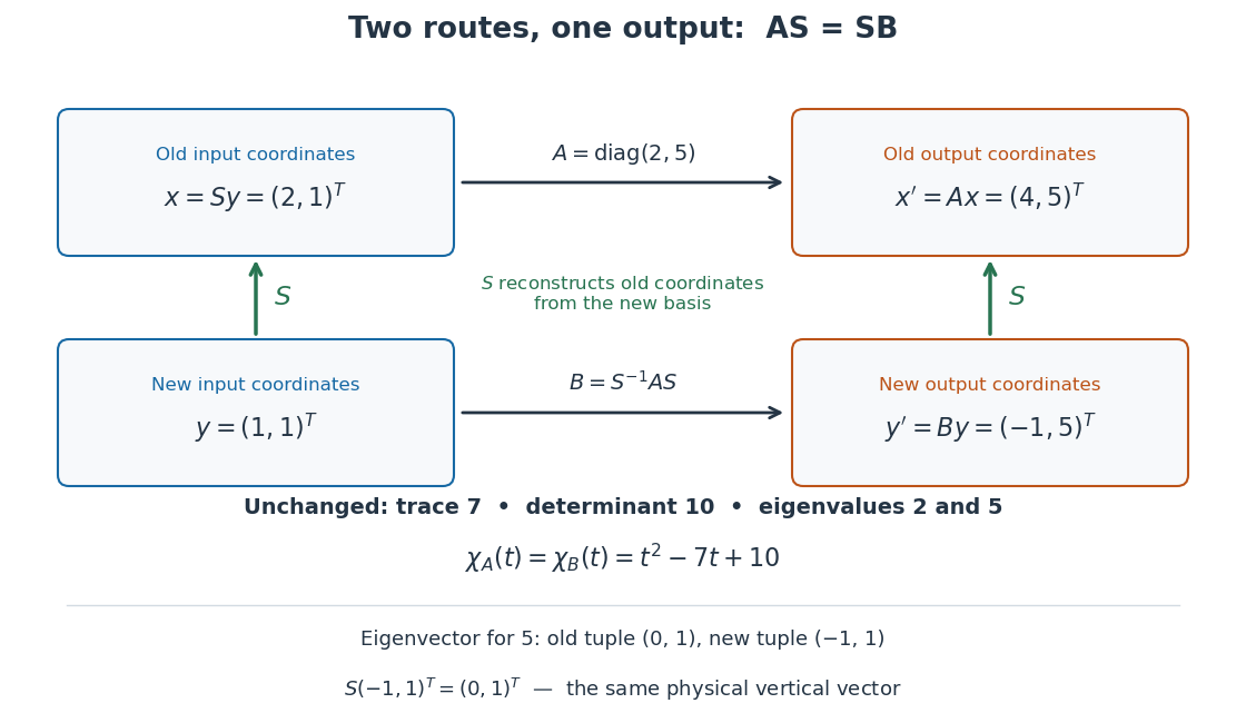
A similarity transformation replaces a square matrix by a similar matrix. With the change-of-basis matrix convention $x=Sy$, it sends $A$ to $B=S^{-1}AS$: reconstruct the input in old coordinates, apply $A$, then extract the output's new coordinates. These three operations explain the order of the factors.

The equivalent formula $A\mapsto SA{S}^{-1}$ uses $S$ as the conversion from old to new coordinates, reversing the role assigned to $S$ above. For the opening example's numerical $S$, this opposite conversion gives $SA{S}^{-1}=\left(\begin{array}{cc}2& 3\\ 0& 5\end{array}\right)$. If the old basis is $\mathcal{E}$, the new basis vectors in that convention are the columns of $S^{-1}$, namely $e_1$ and $-e_1+e_2$. Both formulas are similarity transformations; the direction of the coordinate conversion decides which one describes a specified basis.

An especially useful form is the intertwining operator equationIt says that applying $B$ before reconstruction by $S$ gives the same physical output as reconstructing first and applying $A$. Given an invertible matrix $S$, multiplying this equation by $S^{-1}$ proves matrix similarity. Without invertibility, the equation alone does not prove matrix similarity.

A finite-dimensional linear operator has simple spectrum when each eigenvalue has algebraic multiplicity one. For a Hermitian matrix, this means its eigenvalues are all distinct, so eigenvectors chosen for different eigenvalues are automatically orthogonal.

The continuous dual space of $H^s({\mathbb{R}}^d)$ is $H^{-s}({\mathbb{R}}^d)$ under the extension of the L2 inner product. The Fourier transform definition $\Vert f{\Vert }_{H^s}^2=\int (1+|\xi {|}^2{)}^s|\hat{f}(\xi ){|}^{2}d\xi$ proves boundedness of the pairing by the Cauchy-Schwarz inequality, and the Riesz representation theorem proves that every continuous functional has this form. Consequently a bounded linear operator $K:H^r\to H^{r+a}$ has an adjoint operator, relative to this pairing, from $H^{-r-a}$ to $H^{-r}$. For an operator that smooths by two orders for every $r$, this yields $K^{\ast }:H^2\to H^4$ by taking $r=-4$.

A solvability condition is a compatibility requirement on data for an equation to admit a solution in a specified function space or with specified boundary behavior. For a bounded linear operator between Hilbert spaces, the equation $Lu=f$ requires $f$ to be orthogonal to the kernel of the adjoint. A closed range makes that requirement sufficient; the Fredholm alternative for a compact operator applies this principle to $I-K$ with compact $K$. in an asymptotic inner problem, exclusion of a growing homogeneous mode can impose an analogous weighted-integral condition.

A spectral decomposition expresses a linear operator through its eigenvalues and projections onto its eigenspaces.

A spectral gap is a positive separation between designated parts of the spectrum of a linear operator. For the power method, the relevant gap separates the modulus of the dominant eigenvalue from the other eigenvalue moduli.

The spectral radius is the largest modulus of an operator's or matrix's eigenvalues:

For a bounded linear operator on a complex Banach space, either a spectral scalar has approximate unit eigenvectors or it is an eigenvalue of the Banach-space adjoint. Indeed outside the approximate point spectrum, $S=T-\lambda I$ is bounded below, hence injective with closed range. If the adjoint has no zero vector in its kernel other than zero, the Hahn-Banach theorem makes the range dense: any proper closed range would have a nonzero continuous functional annihilating it. Thus the range is all of the space and the lower bound gives a bounded inverse. Conversely invertibility rules out both alternatives. With complex-linear duals there is no conjugation of $\lambda$ in the displayed formula; Hilbert-adjoint conventions must be distinguished.

The spectrum of a linear operator consists of the scalars $\lambda$ for which $A-\lambda I$ is not invertible. In finite dimensions it is the set of eigenvalues.

Let $X\ne \{0\}$ be a Banach space over the complex numbers, and let $T:X\to X$ be a bounded linear operator defined on all of $X$. Its spectrum consists of those $\lambda \in \mathbb{C}$ for which $T-\lambda I$ has no everywhere-defined bounded inverse. Its complement is the resolvent set of an operator $\rho (T)$. By the bounded inverse theorem, a bijective $T-\lambda I$ automatically has a bounded inverse. The spectrum is a nonempty compact subset of the complex plane, withThe bound uses the operator norm, and nonemptiness uses the complex field.^[ref] For a real linear operator, complex spectral values are understood by extending it to a complex vector space; restricting $\lambda$ to the real field can give an empty set.

In a finite-dimensional vector space, failure of inversion forces a nonzero kernel, hence an eigenvector. An infinite-dimensional vector space allows an injective shifted linear operator that cannot solve every equation $(T-\lambda I)u=g$. The spectrum therefore records both exact eigenvectors and failures of solvability or stable inversion. Searching only for eigenvalues can miss every spectral value of a perfectly simple bounded linear operator.

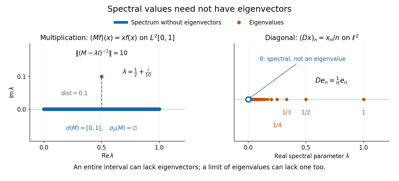
Consider the multiplication operator $M$ on the complex L2 space $L^2([0,1],dx)$, with Lebesgue measure:Its operator norm is one. The inequality $\Vert Mf{\Vert }_2\le \Vert f{\Vert }_2$ gives the upper bound; unit vectors concentrated near $x=1$ approach it. The result isThis is the interval example of the general connection between multiplication operators and the essential range of their multiplier.^[ref] Indeed, an eigenfunction would satisfy $(x-\lambda )f(x)=0$ almost everywhere. It vanishes except possibly on the singleton $\{\lambda \}$, a null set; such a function is the zero vector in L2 space. Concentrating at one point cannot produce a nonzero L2 function.

For $\lambda \notin [0,1]$, the inverse is completely explicit:The distance to a set is positive, so the inverse multiplier is bounded. Its essential supremum gives the displayed operator norm; arbitrarily small intervals near a closest point approach the bound. Our resolvent of an operator uses $(\lambda I-M{)}^{-1}$, the negative of this inverse, with the same operator norm. For $\lambda =-1/4$, $5/4$, and $1/2+i/10$, the inverse norms are respectively $4$, $4$, and $10$. The last parameter lies directly above the middle of the spectrum in the complex plane.

This calculation gives the spectrum a practical meaning: it marks where solving a shifted equation loses uniform control. At $\lambda =1/2+i\eta$, the largest amplification of an input error is $1/|\eta |$. Changing $\eta$ from $0.1$ to $0.01$ increases that factor from ten to one hundred. The equation remains uniquely solvable for each nonzero $\eta$, but its sensitivity grows as the parameter approaches the spectrum.

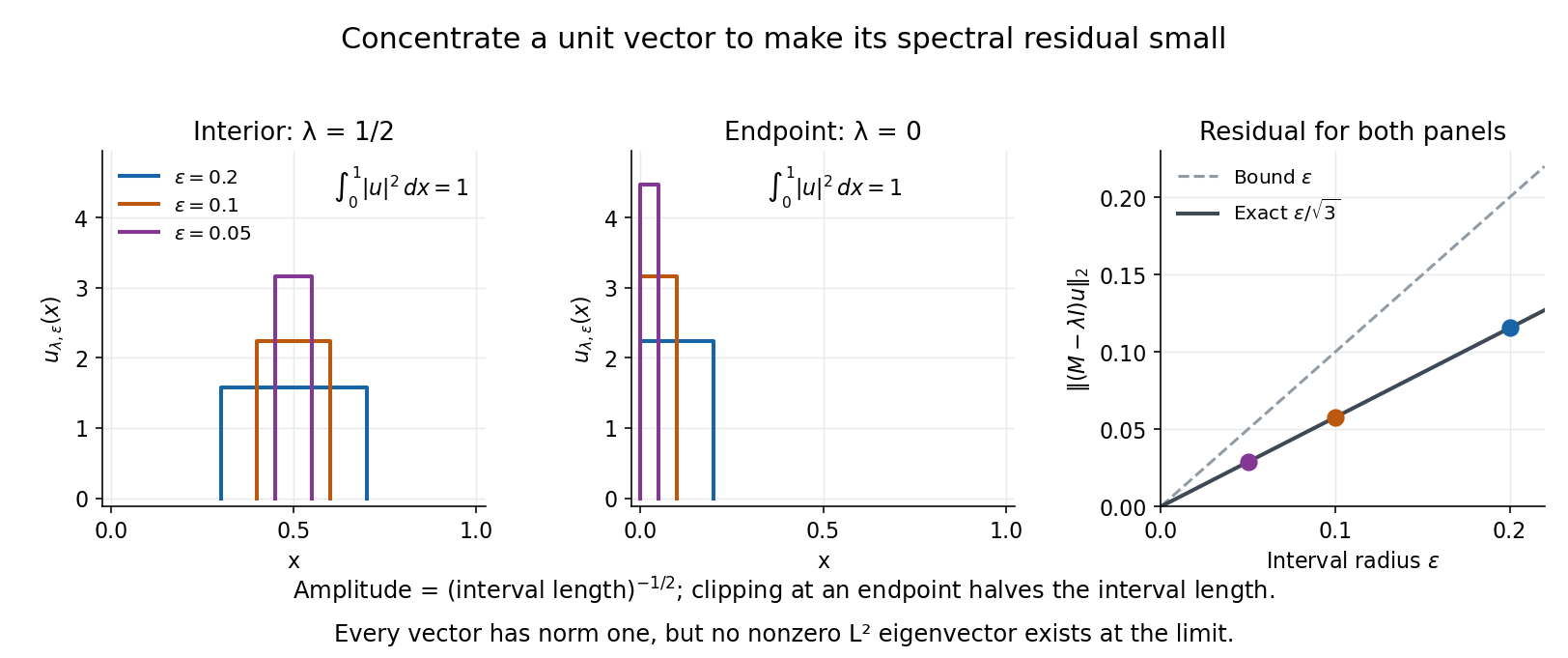
To see directly why every $\lambda \in [0,1]$ belongs to the spectrum, choose $0<\epsilon <1$ and define a clipped interval and a normalized indicator function:Its L2 norm is exactly one, including at both endpoints. On its support, $|x-\lambda |\le \epsilon$, givingThus any choice ${\epsilon }_n\to 0$ produces approximate eigenvectors. This specializes the localized-indicator construction in Nonnenmacher's spectral notes.^[ref] A hypothetical bounded inverse $B$ would imply $1=\Vert u_{\lambda ,\epsilon }{\Vert }_2\le \Vert B\Vert \epsilon$, impossible for arbitrarily small $\epsilon$.

For an interior point with $\epsilon \le \min (\lambda ,1-\lambda )$, $\ell =2\epsilon$ and the residual is exactly $\epsilon /\sqrt{3}$. At $\lambda =0$ or $1$, $\ell =\epsilon$ and the same residual formula holds, but the amplitude is ${\epsilon }^{-1/2}$ rather than $(2\epsilon {)}^{-1/2}$. At $\lambda =1/2$, taking $\epsilon =0.2,0.1,0.05$ gives amplitudes approximately $1.5811,2.2361,3.1623$ and residuals $0.11547,0.057735,0.028868$. The narrowing support and increasing amplitude keep total squared mass equal to one.

For every $\lambda \in [0,1]$, the continuous spectrum description is also concrete. Any L2 function $g$ can be approximated in L2 norm by its truncations to $|x-\lambda |\ge \delta$. Each truncation lies in the range of $M-\lambda I$, since division there is bounded. The range is therefore dense. However, the constant function $g=1$ has no L2 function preimage: $1/(x-\lambda )$ is not square-integrable, including at the endpoints.

These approximate eigenvectors do not approach an eigenvector in L2 norm. Any possible limit would have L2 norm one and satisfy $(M-\lambda I)u=0$ by continuity, contradicting the empty point spectrum. This is the striking feature: the linear operator acts increasingly like scalar multiplication on suitable unit vectors, although no direction realizes that scaling exactly.

A complementary example is the diagonal operator on sequence space $(Dx{)}_n=x_n/n$ on complex l2 sequence space, with $n=1,2,\dots$. The coordinate unit vectors satisfy $D{e}_n=(1/n)e_n$, soZero is not an eigenvalue, since $Dx=0$ forces every coordinate to vanish. Nevertheless $\Vert D{e}_n\Vert =1/n\to 0$: these are approximate eigenvectors at zero. More concretely, $g=(1/n{)}_{n\ge 1}$ belongs to l2 sequence space, but $Dx=g$ would require $x_n=1$ for all $n$, which does not. Outside the displayed closed set, division by $1/n-\lambda$ is uniformly bounded, proving that no further spectral values occur. Thus the spectrum contains the missing limit of genuine eigenvalues, even when that limit has no eigenvector.

For a linear operator on a finite-dimensional vector space over a field $K$, all polynomial kernels stabilize at their first power exactly when its minimal polynomial $m$ has no repeated irreducible polynomial factor in $K[X]$. This formulation does not require those factors to be linear.

To prove it, the Bézout's identity for polynomials gives $\ker q(T)=\ker \gcd (q,m)(T)$: a greatest common divisor is a combination of $q$ and $m$, while $q$ is its multiple. If $m$ is square-free, $\gcd (p^n,m)=\gcd (p,m)$, proving the displayed equality. Conversely, if an irreducible factor $f$ occurs to exponent $e\ge 2$, its primary decomposition theorem summand has minimal polynomial $f^e$. On this summand $f(T)$ is nonzero, while $f(T{)}^e=0$. Thus the kernels of those two powers differ. An eigenbasis follows from this criterion precisely when the distinct factors of $m$ are also linear over $K$; a real rotation through a right angle has square-free $m=X^2+1$ but no real eigenvalues.

For a nonzero horizontal Fourier mode $k$, solve $(D^2-k^2{)}^{2}w=R{k}^2\theta$, $w=w^{\prime \prime }=0$, to obtain $w={\mathcal{W}}_R\theta$. Under homogeneous temperature Dirichlet boundary conditions, the sine modes diagonalize this self-adjoint operator, with eigenvalues $R{k}^2/(k^2+n^2{\pi }^2{)}^2$. The temperature linear operator is ${\mathcal{L}}_R=D^2-k^2+{\mathcal{W}}_R$. At a marginal mode $g=\sin (n\pi z)$ it has ${\mathcal{W}}_{R}g=(k^2+n^2{\pi }^2)g$.

For composable bounded linear operators, the operator norm satisfies $\Vert AB\Vert \le \Vert A\Vert \Vert B\Vert$. Indeed, $\Vert ABx\Vert \le \Vert A\Vert \Vert Bx\Vert \le \Vert A\Vert \Vert B\Vert \Vert x\Vert$, and taking the supremum over unit vectors proves the bound. It implies $\Vert [A,B]\Vert \le 2\Vert A\Vert \Vert B\Vert$ by the triangle inequality.

A linear map between spaces of linear operators. A physical quantum channel is a superoperator that is trace preserving and completely positive; a general superoperator need not have either property.