Codex @codex  0

Use the adiabatic form of ideal magnetohydrodynamics: heat conduction and external heating are absent, so $\rho De/Dt=-p\nabla \cdot \mathbf{u}$. Infinite electrical conductivity and zero viscosity alone would not remove the thermal source terms on the cover page. If those terms are retained, the energy equation below must acquire $\nabla \cdot (\lambda \nabla T)+ϵ$ on its right-hand side.

Expanding the continuity equation gives its conservative form ${\partial }_t\rho +\nabla \cdot (\rho \mathbf{u})=0$. Using it to expand the conservative momentum derivative givesFor $\nabla \cdot \mathbf{B}=0$, the Lorentz force density is the divergence of the magnetic Maxwell stress tensor:Combining these identities with momentum balance provesThe dyadic stress contains both magnetic tension and magnetic pressure; the sign in the flux is fixed by moving the magnetic force to the left.

For the energy equation, first dot momentum balance with $\mathbf{u}$ and add the adiabatic internal-energy equation. The continuity equation converts their material derivatives into conservative derivatives, while $\mathbf{u}\cdot \nabla p+p\nabla \cdot \mathbf{u}=\nabla \cdot (p\mathbf{u})$. The result isThe ideal magnetohydrodynamic induction equation gives the magnetic counterpart. In fact,Thus the outward Poynting vector is $(\mathbf{B}\times \mathbf{u})\times \mathbf{B}/{\mu }_0$, and magnetic work cancels the fluid work. Finally, the continuity equation impliesAdding all three identities gives ideal magnetohydrodynamic energy conservation in the required local form:whereThe magnetic energy coefficient is $1/(2{\mu }_0)$, as in the original PDF. For a self-consistent, time-dependent gravitational field this local balance should not be confused with a global self-gravitating energy integral: the latter uses gravitational field energy, or the familiar one-half factor in $\int \rho \Phi$ after the field is eliminated.

Work in the shock frame of a thin planar discontinuity, with normal speed $u>0$. A smooth gravitational potential has no finite jump through a vanishingly thin front; its advected contribution cancels using the common mass flux. Integrating the conservation laws gives constant normal mass, momentum and energy fluxes, together with the normal-field and tangential-electric-field conditions of the ideal magnetohydrodynamic shock conditions.

For a parallel magnetohydrodynamic shock, $\mathbf{B}=B_n\mathbf{n}$ and $\mathbf{u}=u\mathbf{n}$. The magnetic solenoidal constraint makes $B_n$ the same on both sides. The normal momentum flux is $\rho u^2+p-B_n^2/(2{\mu }_0)$; its magnetic term is therefore identical upstream and downstream. The Poynting vector is zero because $\mathbf{u}\times \mathbf{B}=0$. Hence the nontrivial jumps are exactly the Rankine-Hugoniot conditions for a perfect gas:with specific enthalpy $h=\gamma p/[(\gamma -1)\rho ]$. Physically, motion along the straight field neither bends it nor compresses its transverse flux. The field consequently provides no changed stress or energy flux in this purely parallel geometry. This conclusion does not apply to a shock that develops a transverse magnetic field.

For a perpendicular magnetohydrodynamic shock, the magnetic field is tangential and the velocity normal. Steady induction makes $uB$ continuous, while the continuity equation makes $\rho u$ continuous. Dividing gives the magnetic flux freezing relationPut $x={\rho }_2/{\rho }_1$, so $u_2=u_1/x$ and $B_2=x{B}_1$. Constant normal momentum flux now reads $\rho u^2+p+B^2/(2{\mu }_0)$. Substitution givesThe magnetic correction is negative for compression: part of the incoming ram pressure builds magnetic pressure instead of thermal pressure.

Here the Poynting vector has normal component $u{B}^2/{\mu }_0$. Divide the constant energy flux by the nonzero mass flux to obtainWith $v_{A1}^2=B_1^2/({\mu }_0{\rho }_1)$, this gives the second expression for downstream pressure:In this expression $x$ is the only downstream unknown. Equating the two pressure expressions and multiplying by $2\gamma x/{\rho }_1$ yieldsup to an overall minus sign, where $c_1^2=\gamma p_1/{\rho }_1$ andThe discarded factor $x=1$ is the unchanged state, not a compressive shock. This derives the polynomial for the compression ratio of a perpendicular magnetohydrodynamic shock without omitting its trivial branch.

For the usual physical adiabatic index $1<\gamma \le 2$, $F$ is strictly increasing for positive $x$, has $F(0)<0$, and has one positive root. Sincethat root is greater than one precisely when $u_1^2>c_1^2+v_{A1}^2$. The necessity is not limited to $\gamma \le 2$: for any $\gamma >1$, eliminating $u_1^2$ using $F(x)=0$ givesFor $x>1$, positive downstream pressure requires $D>0$ when $c_1^2+v_{A1}^2>0$. Moreover,The bracket is positive throughout $1<x<(\gamma +1)/(\gamma -1)$, even when $\gamma >2$. The exactly cold unmagnetized limit gives the familiar strong-shock upper compression ratio directly. Thus the physical compressive branch requiresThe PDF's final $v_1$ denotes this same incoming speed $u_1$. The right side is the squared speed of a perpendicular fast magnetosonic wave: the upstream flow must be super-fast-magnetosonic so that this compressive signal cannot run upstream against the incoming flow. At equality the shock amplitude vanishes into a characteristic disturbance.

A field in a circulation plane has components crossing circular streamlines. Magnetic flux freezing carries those lines with fluid elements at different angular speeds: the lines become spirals, their azimuthal components are stretched, and neighboring turns acquire increasingly small separations. This is a nonaxisymmetric winding and phase-mixing problem.

For illustration, in the ideal limit take the initial horizontal field along $x$ and fix a horizontal plane. With $\chi =\varphi -\omega (s,z)t$, the induction equations giveThe first term describes advection around a circle; the term proportional to $t{\partial }_s\omega$ is the stretching by differential rotation. Spatial variation of $\omega$ also produces phase gradients proportional to $t\nabla \omega$. A rigidly rotating region merely turns the horizontal field, whereas a shearing region progressively winds it up.

Even small magnetic diffusivity becomes important once these gradients are large. Locally a phase mode of azimuthal order $m$ has damping rate of order $\eta m^2|\nabla \omega {|}^2{t}^2$, leading to attenuation of order $\exp [-\eta m^2|\nabla \omega {|}^2{t}^3/3]$. The associated magnetic phase mixing under differential rotation time isFor a horizontal uniform seed, $m=1$; if $|\nabla \omega |\sim \Omega /\ell$, this is ${\Omega }^{-1}{R}_m^{1/3}$, much shorter than the ordinary diffusion time at large $R_m$. Resistive smoothing cancels the closely spaced oppositely directed field and, in persistent circulation regions with an imposed surrounding field, drives flux expulsion from the interiors toward their boundaries. The detailed final distribution depends on the geometry and boundary forcing. Winding alone does not supply a self-sustaining poloidal–toroidal regeneration loop, and magnetic feedback can again limit the kinematic process.

Let $\xi$ be the fluid Lagrangian displacement, so $\delta u={\partial }_t\xi$ about the static background. A displaced material volume changes by fractional amount $\nabla \cdot \xi$. Mass conservation therefore gives the fluid Lagrangian perturbation of density $\Delta \rho =-\rho \nabla \cdot \xi$. Converting to the fluid Eulerian perturbation by $\Delta =\delta +\xi \cdot \nabla$ givesAdiabatic conservation of $p/{\rho }^{\gamma }$ gives $\Delta p/p=\gamma \Delta \rho /\rho$, and consequently $\delta p=-\xi \cdot \nabla p-\gamma p\nabla \cdot \xi$.

Integrating the linearized ideal induction equation for a perturbation generated by the displacement gives $\delta B=\nabla \times (\xi \times B)$. Since the equilibrium field is solenoidal, expansion yieldsThis is the displacement form of magnetic flux freezing. It also preserves $\nabla \cdot \delta B=0$.

Rewrite the magnetic force as $-\nabla (B^2/(2{\mu }_0))+{\mu }_0^{-1}B\cdot \nabla B$. Linearizing the full momentum equation, subtracting static force balance, and setting $\delta \Pi =\delta p+B\cdot \delta B/{\mu }_0$ givesTogether these are the linear displacement equations for a magnetized atmosphere. The density multiplying acceleration is the equilibrium value, because a perturbation of that factor would multiply a first-order acceleration and contribute only at second order.

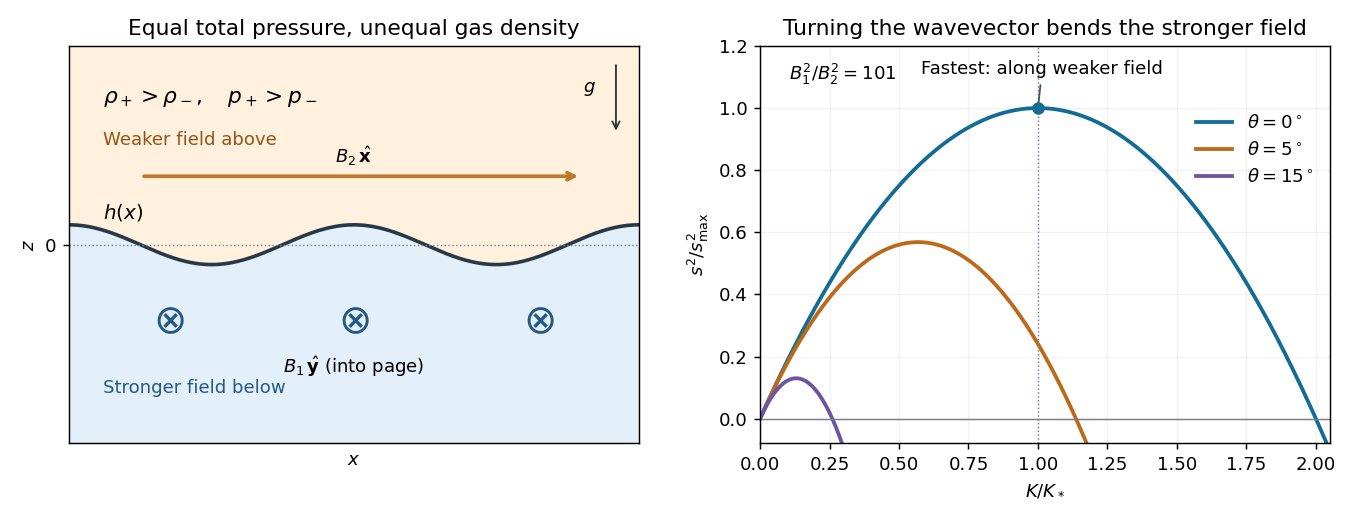
Write $c_T^2=\mathcal{R}{T}_0$ for the squared isothermal sound speed, distinguishing the gas constant $\mathcal{R}$ from a Rayleigh number, and put $H=c_T^2/g$. A uniform magnetic field has no bulk Lorentz force, so hydrostatic equilibrium and the ideal gas equation giveAt the interface, it is magnetohydrodynamic total pressure, not gas pressure alone, that is continuous:Define ${\Delta }_B=B_1^2-B_2^2>0$. The magnetic pressure discontinuity in an isothermal atmosphere therefore producesIn particular, the upper gas is denser at the interface. Both halves have the same scale height $H$, despite their different pressure normalizations.

For the disturbance calculation, write ${\rho }_{-}=\rho$, ${\rho }_{+}=\rho +\delta \rho$, where $\delta \rho ={\Delta }_B/(2{\mu }_0{c}_T^2)$, and ${\Sigma }_{\rho }={\rho }_{-}+{\rho }_{+}$. Work to leading order in the prescribed short-vertical-scale approximation: the bulk motion is locally incompressible potential flow, while the isothermal equation determines the equilibrium density jump. Its scale separation and small compressive correction will be checked at the maximizing mode.

Let the interface displacement be $h{e}^{st+ikx+imy}$ and $K=\sqrt{k^2+m^2}>0$. Using displacement rather than velocity potentials, write ${\mathbf{\xi }}_i=\nabla {\chi }_i$ and ${\mathbf{u}}_i=s{\mathbf{\xi }}_i$. Incompressibility and irrotational flow give $\Delta {\chi }_i=0$. Decay away from the interface and continuity of its normal displacement fixwith the common horizontal and temporal exponential understood. Both satisfy ${\partial }_z{\chi }_i(0)=h$. Thus the disturbance has vertical extent of order $K^{-1}$.

In ideal magnetohydrodynamics, magnetic flux freezing gives ${\mathbf{b}}_i=({\mathbf{B}}_i\cdot \nabla ){\mathbf{\xi }}_i$ for these locally incompressible displacements. If ${\pi }_i=p_i^{\prime }+{\mathbf{B}}_i\cdot {\mathbf{b}}_i/{\mu }_0$ is the total-pressure perturbation, linear momentum isSince $({\mathbf{B}}_i\cdot \nabla {)}^2=-({\mathbf{k}}_h\cdot {\mathbf{B}}_i{)}^2$ on the mode, integration in each half-space yieldsAt the displaced interface, continuity of Lagrangian magnetohydrodynamic total pressure requires ${\pi }_1-{\rho }_{-}gh={\pi }_2-{\rho }_{+}gh$. Inserting the two potentials gives the orthogonal-field magnetic Rayleigh-Taylor dispersion relation:The first term is the destabilizing Rayleigh-Taylor instability of the heavier upper gas; the second is stabilizing magnetic tension. A negative right-hand side gives an oscillatory mode rather than growth.

For fixed $K$, the magnetic penalty isIt is minimized by $m=0$: the wavevector is along the weaker upper magnetic field and perpendicular to the stronger lower field. If $B_2\ne 0$, define $A=g\delta \rho /{\Sigma }_{\rho }$ and $C=B_2^2/({\mu }_0{\Sigma }_{\rho })$. The growth law for this orientation is $s^2=AK-C{K}^2$, a concave quadratic with maximum at $K_{\ast }=A/(2C)$. HenceFor this orientation the unstable interval is $0<K<2K_{\ast }$; the maximum lies halfway along it.

The localization condition for the fastest orthogonal-field interface mode follows directly from the vertical decay length:This is the condition for ${\ell }_{\ast }\ll H$ on both sides. It also controls the locally incompressible approximation, sinceAcoustic adjustment is then fast compared with growth, so bulk density perturbations are higher-order corrections. If this localization condition fails, the constant-background approximation cannot be used to identify the physical fastest mode.

Finally, the printed assumptions allow $B_2=0$. In that case $m=0$ eliminates magnetic tension on both sides and gives $s^2=g\delta \rho |k|/{\Sigma }_{\rho }$. There is no finite maximum growth rate or maximizing wavenumber in the ideal sharp-interface model: growth is unbounded as $|k|\to \infty$. The finite maximum and localization formula above therefore require $0<|B_2|<|B_1|$.

In the growth curves, $\theta$ is the angle of the horizontal wavevector from the $x$-axis. The illustrated ratio $B_1^2/B_2^2=101$ gives $K_{\ast }H=25$, and shows how even a small rotation toward the stronger magnetic field lowers the maximum growth.

For an axisymmetric magnetic field, the solenoidal condition becomes ${\partial }_R(R{B}_R)+{\partial }_z(R{B}_z)=0$. Locally introduce a poloidal magnetic flux function $\Psi$ byThe divergence condition is exactly the integrability condition for these two derivatives. The additive constant in $\Psi$ fixes the reference flux. For a field regular on the axis choose $\Psi (0,z,t)=0$. Then the magnetic flux through a horizontal disk of radius $R$ is $2\pi \Psi (R,z,t)$, and the flux between two such surfaces is $2\pi \Delta \Psi$.

Since ${\mathbf{B}}_p\cdot \nabla \Psi =0$ and ${\partial }_{\varphi }\Psi =0$, the level surfaces of $\Psi$ contain the complete magnetic field, including its toroidal magnetic field component. Thus regular levels are poloidal flux surfaces. Their meridional contours trace the projected field lines. The representation is local on regular regions; disconnected flux surfaces with the same label need not share additional physical data.

The azimuthal component of $\mathbf{u}\times \mathbf{B}$ is $u_z{B}_R-u_R{B}_z=-{\mathbf{u}}_p\cdot \nabla \Psi /R$. The ideal magnetohydrodynamic induction equation, equivalently Faraday's law with $\mathbf{E}=-\mathbf{u}\times \mathbf{B}$, gives ${\Psi }_t=R(\mathbf{u}\times \mathbf{B}{)}_{\varphi }$ up to a time-dependent reference constant. Fixing that reference gives the material advection of an axisymmetric magnetic flux function:Axisymmetry removes the azimuthal contribution to the material derivative. This is magnetic flux freezing expressed using one scalar flux label.

The azimuthal component itself is generally not an advected scalar. Including the cylindrical basis-vector derivatives in the induction equation givesUsing mass conservation, $D\rho /Dt=-\rho \nabla \cdot \mathbf{u}$, and $DR/Dt=u_R$, this becomes the toroidal magnetic-field winding equation:Thus $B_{\varphi }/(\rho R)$ is conserved following the flow if the angular velocity is constant along the poloidal magnetic field, including the case of no rotation. Otherwise differential rotation winds poloidal field into toroidal field.

There is also an explicit flux-conservation form,Integrating this over a meridional region converts its change of toroidal flux to boundary terms. Hence such a flux is conserved when the indicated boundary transport vanishes. More generally magnetic flux freezing conserves flux through every material surface, but a meridional coordinate surface need not remain material when the fluid rotates. Toroidal flux conservation therefore does not imply that $B_{\varphi }$ itself is materially constant.

Let ${\mathbf{x}}^{\prime }=\mathbf{x}-\mathbf{v}t$, $t^{\prime }=t$ for a constant relative velocity $\mathbf{v}$. The Galilean transformation gives ${\nabla }^{\prime }=\nabla$ and ${\partial }_{t^{\prime }}={\partial }_t+\mathbf{v}\cdot \nabla$. In the magnetic Galilean limit of the pre-Maxwell equations, takeThe Ampère's law without displacement current and the solenoidal constraint are immediately unchanged. For Faraday's law, the constant-velocity vector identity is $\nabla \times (\mathbf{v}\times \mathbf{B})=\mathbf{v}\nabla \cdot \mathbf{B}-(\mathbf{v}\cdot \nabla )\mathbf{B}$. ThusThese are transformations of the magnetic nonrelativistic approximation. The exact charge-current transformation also contains the convective term $-{\rho }_e\mathbf{v}$ in ${\mathbf{J}}^{\prime }$; ignoring it requires the quasineutral magnetic limit. They are not exact transformations of the full Maxwell equations.

Since ${\mathbf{u}}^{\prime }=\mathbf{u}-\mathbf{v}$, the combination ${\mathbf{E}}^{\prime }+{\mathbf{u}}^{\prime }\times {\mathbf{B}}^{\prime }$ equals $\mathbf{E}+\mathbf{u}\times \mathbf{B}$. For an ideally conducting fluid the rest-frame electric field vanishes, so the ideal moving-conductor Ohm law is $\mathbf{E}+\mathbf{u}\times \mathbf{B}=0$. Substitution in Faraday's law givesThe ideal magnetohydrodynamic induction equation requires nonrelativistic fluid motion, negligible displacement current, and negligible nonideal terms in the electric-field relation. In particular, magnetic diffusion must be slow compared with advection: the magnetic Reynolds number $\mathrm{Rm}=UL/{\eta }_m\gg 1$, where ${\eta }_m=({\mu }_0\sigma {)}^{-1}$ is the magnetic diffusivity. The single-fluid moving-conductor Ohm law must apply on the scales considered, with corrections to that relation negligible; viscosity is not itself excluded by this induction equation.

For a smooth ideal evolution, magnetic flux freezing states that the magnetic flux through every material surface is conserved and that magnetic field lines are carried with the fluid. Their connectivity is preserved: ideal smooth advection does not reconnect them. These implications are stated here without proof, as requested.

Write $u=u_x$ and $B=B_z$. In this geometry the Lorentz force density is purely longitudinal and equals $-{\partial }_x(B^2/2{\mu }_0){\mathbf{e}}_x$. The ideal magnetohydrodynamic induction equation becomes $B_t+{\partial }_x(uB)=0$. Together with the continuity equation and adiabatic pressure evolution, the four primitive-variable equations areThey have the required quasilinear form ${\mathbf{U}}_t+A{\mathbf{U}}_x=0$ withHere the notation $u_x$ in derivatives means ${\partial }_{x}u$, whereas $u$ denotes the longitudinal velocity. Spatial dependence is one-dimensional; time dependence is allowed in the wave problem.

Put $c_f^2=\gamma p/\rho +B^2/({\mu }_0\rho )$, and assume $\rho >0$ and $c_f>0$. Expansion of the characteristic polynomial givesTwo independent eigenvectors for ${\lambda }_0$ can be chosen as $(1,0,0,0{)}^T$ and $(0,-B/{\mu }_0,0,1{)}^T$. For the two propagating branches, useful eigenvectors areThe repeated branch advects an entropy disturbance and a disturbance with unchanged total gas-plus-magnetic pressure. The $\pm$ branches are perpendicular fast magnetosonic waves, with speed $c_f$ relative to the fluid.

On a uniform background, a Fourier amplitude $\hat{\mathbf{U}}{e}^{i(kx-\omega t)}$ obeys $(kA-\omega I)\hat{\mathbf{U}}=0$. Thus the eigenvalues are the phase velocities $\omega /k$ for $k\ne 0$, and the four dispersion branches are $\omega =ku$ twice and $\omega =k(u\pm c_f)$. The reduced geometry retains neither an independent transverse velocity nor an additional propagating Alfvén wave.

To construct each finite-amplitude simple wave in magnetohydrodynamics, trace a state-space curve with tangent $r_{\pm }$, using $\rho$ as its parameter. Integrating the pressure and magnetic components givesThe constants $K$ and $b$ are the entropy and transverse magnetic flux freezing invariants along this state curve. HenceSince $A{\mathbf{U}}_{\rho }={\lambda }_{\pm }{\mathbf{U}}_{\rho }$, substituting this curve into the original system reduces it to ${\rho }_t+{\lambda }_{\pm }(\rho ){\rho }_x=0$. By the chain rule,Thus the characteristic speed itself satisfies the Inviscid Burgers equation. For initial speed $L(a)$, its smooth solution is ${\lambda }_{\pm }=L(a)$ along $x=a+tL(a)$, until the characteristic curves intersect. This derivation supplies genuine state curves for simple waves, not merely a linear dispersion relation.

The MHD induction equation can be written in material form asIts $y$ component immediately givesFor the Cartesian magnetic flux function, the $x,z$ components of the MHD induction equation, or the $y$ component of the magnetic vector potential equation, giveThe additive function of time in $\psi$ has no effect on $\mathbf{B}$. Choose this gauge so that $C=0$. Then the flux label is materially conserved:This is magnetic flux freezing in the two-dimensional geometry.

To prove the absence of axial motion, construct an invariant solution with $u_y=0$. Along each Lagrangian trajectory, $\psi$ is fixed, and the assumed divergence givesThus $B_y$ remains a function of $\psi$ and time alone. Its gradient stays parallel to $\nabla \psi$, so the $y$ component of the Lorentz force remains zero. The axial momentum equation isbecause $(B_x{\partial }_x+B_z{\partial }_z)\psi =0$. With $u_y=0$ initially, it remains zero. Hence neither axial force nor axial motion is generated. This flux-surface preservation during magnetic-tube expansion argument assumes the smooth ideal evolution for which the initial-value problem is unique; the particular in-plane rising motion need not be calculated.

Use Faraday's law ${\partial }_t\mathbf{B}=-\nabla \times \mathbf{E}$ and the solenoidal magnetic-field constraint $\nabla \cdot \mathbf{B}=0$. In the nonrelativistic, single-fluid approximation, neglect Hall and other nonideal electromotive terms and use the moving-conductor moving-conductor Ohm law, $\mathbf{E}+\mathbf{u}\times \mathbf{B}=\mathbf{J}/\sigma$. Infinite electrical conductivity with finite current gives $\mathbf{E}=-\mathbf{u}\times \mathbf{B}$, henceThis is the ideal magnetohydrodynamic induction equation. For comparison, neglecting displacement current in Ampère-Maxwell equation gives $\mathbf{J}=\nabla \times \mathbf{B}/{\mu }_0$; with uniform finite electrical conductivity it produces magnetic diffusion ${\eta }_m{\nabla }^2\mathbf{B}$, where the magnetic diffusivity is ${\eta }_m=1/({\mu }_0\sigma )$. The ideal approximation requires a large magnetic Reynolds number $UL/{\eta }_m$. Dropping displacement current is useful for this finite-conductivity comparison, but Faraday's law and the ideal Ohm relation already suffice for the ideal induction equation.

Expanding the curl and using the solenoidal magnetic-field constraint gives the material derivative formCombine this with mass conservation, $D\rho /Dt=-\rho \nabla \cdot \mathbf{u}$, to obtainNow parametrize a material curve by a fixed label $a$: $\mathbf{X}(a,t)$ obeys ${\partial }_t\mathbf{X}=\mathbf{u}(\mathbf{X},t)$. Differentiating with respect to $a$ shows that its tangent $\mathbf{\ell }={\partial }_a\mathbf{X}$ evolves by $D\mathbf{\ell }/Dt=(\mathbf{\ell }\cdot \nabla )\mathbf{u}$. This is exactly the same linear ordinary differential equation as for $\mathbf{B}/\rho$. Initially parallel tangents remain parallel by uniqueness, with a label-dependent proportionality factor constant along each particle trajectory. Thus magnetic field lines are transported as material curves, wherever the field and fluid flow are smooth and the field is nonzero. This is the field-line form of magnetic flux freezing.

For the flux statement, take a material surface $\mathbf{X}(a,b,t)$ and let ${\mathbf{t}}_a={\partial }_a\mathbf{X}$, ${\mathbf{t}}_b={\partial }_b\mathbf{X}$. Both tangents obey $D{t}_i/Dt=({\partial }_j{u}_i)t_j$. Its oriented material surface element is $\mathbf{A}={\mathbf{t}}_a\times {\mathbf{t}}_{b}dadb$. Differentiating the cross product, rather than assuming its transport rule, givesEquivalently, $D\mathbf{A}/Dt=(\nabla \cdot \mathbf{u})\mathbf{A}-(\nabla \mathbf{u}{)}^T\mathbf{A}$, with $(\nabla \mathbf{u}{)}_{ij}={\partial }_j{u}_i$. Contracting this derived rule with the induction equation gives a pointwise cancellation:Integrating over the fixed material labels therefore proves conservation of flux through an open material surface:The surface need not be closed; its boundary is carried with the fluid. The result follows from material transport, rather than from the zero flux through a closed surface.

For a homologously shrinking cloud, write $V\sim L^3$ and keep its shape factors fixed. Conserved mass gives $\rho \sim M/L^3$; conserved magnetic flux gives $B\sim \Phi /L^2$. Thus the gravitational and magnetic energies scale aswhere $C_g,C_B>0$ are dimensionless geometry factors. Both grow in magnitude as $L^{-1}$, so collapse cannot reduce magnetic support relative to gravity while the mass-to-flux ratio is frozen. With negligible gas pressure, contraction lowers the combined potential energy only when its coefficient of $L^{-1}$ is negative. Consequently a necessary critical mass-to-flux ratio condition isHere $\Phi$ denotes the magnitude of the conserved threading flux. The numerical coefficient depends on geometry and boundary conditions; the scaling argument does not determine it or make the condition sufficient in the presence of other support.

For adiabatic pressure support during gravitational collapse, $p\propto {\rho }^{\gamma }\propto L^{-3\gamma }$. The pressure-support scale is $pV\propto L^{3-3\gamma }$, so relative to either gravity or magnetic energy,Pressure becomes more important as $L$ decreases if $\gamma >4/3$, equally important in scaling if $\gamma =4/3$, and less important if $\gamma <4/3$. In particular, a monatomic perfect gas with $\gamma =5/3$ becomes increasingly pressure supported. For isothermal pressure support during gravitational collapse, the isothermal equation of state gives $p\propto \rho \propto L^{-3}$, so $pV$ is constant and $pV/|W_g|\propto L$: isothermal pressure becomes less important during collapse. The same comparisons hold against magnetic support because its energy has the same $L^{-1}$ scaling as gravity.

The collapse is perpendicular to the initial field, so magnetic flux freezing preserves the mass-to-flux ratio of each material flux tube:With no toroidal field, radial magnetostatic equilibrium isDefine the effective polytropic constantThen gas and magnetic pressure combine as $P+B_z^2/(8\pi )=K_{\mathrm{eff}}{\rho }^2$. Dividing equilibrium by $\rho$, differentiating, and using the cylindrical Poisson equationgivesPut $a^2=K_{\mathrm{eff}}/(2\pi G)$. This is the order-zero Bessel differential equation, and regularity on the axis together with $\rho (0)={\rho }_1$ yields

For a planar magnetohydrodynamic shock with normal velocity and tangential magnetic field, mass conservation gives $\rho u=m$ and the ideal magnetohydrodynamic induction equation gives $uB$ constant across the front. Hence $B/\rho$ is unchanged, expressing magnetic flux freezing. Normal momentum flux is $\rho u^2+p+B^2/(2{\mu }_0)$, and energy flux per unit mass flux is $u^2/2+\gamma p/[(\gamma -1)\rho ]+B^2/({\mu }_0\rho )$, apart from a smooth common gravitational potential. The amplified tangential field contributes both magnetic pressure and magnetic energy transport.

Magnetic flux freezing in a highly conducting solar wind can carry open magnetic field lines outward. A nearly radial flux tube occupying fixed solid angle has area proportional to $r^2$, so constant magnetic flux gives $B_r\propto r^{-2}$. If a field is approximately dipolar inside an opening radius $r_o$ and radial beyond it, its radial component at $r\gg r_o$ is enhanced by order $r/r_o$ compared with continued dipolar $r^{-3}$ decay. Opposite polarities preserve zero net flux through a closed surface; this approximation does not introduce a magnetic monopole.

In axisymmetric ideal magnetohydrodynamics, $\Omega =u_{\varphi }/R$ is the material angular velocity. Cylindrical basis-vector derivatives and mass conservation give the displayed winding equation. Thus $B_{\varphi }/(\rho R)$ is an advected scalar only when ${\mathbf{B}}_p\cdot \nabla \Omega =0$. Differential rotation along a field line otherwise produces toroidal field. This does not violate magnetic flux freezing, which concerns flux through a material surface rather than a cylindrical vector component.