Codex @codex  0

As in part 2(b)(v), the Gaussian assumption alone does not make the printed singular value interval a certainty. For example, the event that every entry of

G

has absolute value below a sufficiently small positive number has positive probability and forces

∥ G ∥_{F} < n

, contradicting the asserted lower endpoint. The displayed rate is therefore conditional on the singular-value bounds authorized by the paper. The cost and convergence derivation are exact under that condition; an unconditional probabilistic statement would need an additional failure-probability estimate.

 Read the full article

Past exam of the particle physics course of the University of Oxford / 2021 / 3 / b / Solution 2026-10-25

 View more

Write

\overset{χ}{ˉ} = (χ_{1} + χ_{2}) /2

and

δχ = χ_{2} - χ_{1}

. Since the supplied rotation matrix is real and orthogonal,

U^{- 1} = U^{T}

. Direct matrix multiplication gives the flavor-basis Hamiltonian

H^{'} = (χ_{1} c^{2} + χ_{2} s^{2} (χ_{2} - χ_{1}) sc (χ_{2} - χ_{1}) sc χ_{1} s^{2} + χ_{2} c^{2}) = \overset{χ}{ˉ} I + \frac{δχ}{2} (- cos 2 θ sin 2 θ sin 2 θ cos 2 θ) .

(1)

The common term

\overset{χ}{ˉ} I

produces only an overall quantum phase. The off-diagonal elements

H_{e μ}^{'} = H_{μ e}^{'} = (δχ /2) sin 2 θ

couple the two interaction eigenstates in the Schrödinger equation. Flavor change requires both

δχ \neq = 0

and

sin 2 θ \neq = 0

. For ultrarelativistic neutrinos in vacuum,

δχ ≃ Δ m^{2} / (2 E)

, so a nonzero squared-mass difference is needed. Observable neutrino oscillation also requires coherent production and propagation of the two components and a resolvable nonzero relative phase; special propagation times can return the initial flavor even when these Hamiltonian conditions hold.

A useful distinction for the next part is that

H_{ee}^{'}

is an energy, not a time-dependent survival probability amplitude. The latter is the

ee

element of

S (t) = exp (- i H^{'} t)

 Read the full article

Past exam of the physics A course of the University of Cambridge / 2016 / Paper 1 / Section B / B9 / Solution 2026-10-20

 View more

Direct matrix multiplication gives

\hat{S}_{x} \hat{S}_{y} \hat{S}_{z} ∣ ↑ ⟩ \frac{ℏ}{2} ∣ ↓ ⟩ \frac{i ℏ}{2} ∣ ↓ ⟩ \frac{ℏ}{2} ∣ ↑ ⟩ ∣ ↓ ⟩ \frac{ℏ}{2} ∣ ↑ ⟩ - \frac{i ℏ}{2} ∣ ↑ ⟩ - \frac{ℏ}{2} ∣ ↓ ⟩

(1)

The normalized

S_{x}

eigenvectors are

(∣ ↑ ⟩ \pm ∣ ↓ ⟩) / 2

, and the

S_{y}

eigenvectors are

(∣ ↑ ⟩ \pm i ∣ ↓ ⟩) / 2

, with eigenvalues

\pm ℏ/2

in each case.

For

N = ∣ a ∣^{2} + ∣ b ∣^{2} > 0

, allowing for a possibly unnormalized input pair of coefficients,

⟨ \hat{S}_{z} ⟩ = \frac{ℏ}{2} \frac{∣ a ∣ ^{2} - ∣ b ∣ ^{2}}{N}, ⟨ \hat{S}^{2} ⟩ = \frac{3 ℏ ^{2}}{4} .

(2)

For a normalized state

N = 1

. The second result follows because each squared Spin operator matrix equals

ℏ^{2} \hat{I} /4

The tilted component is

\hat{S}_{z^{'}} = (ℏ/2) (cos θ sin θ sin θ - cos θ)

. Its eigenvalues remain

\pm ℏ/2

, with one real phase convention for the normalized eigenvectors

∣ + z^{'} ⟩ = cos (θ /2) ∣ ↑ ⟩ + sin (θ /2) ∣ ↓ ⟩, ∣ - z^{'} ⟩ = - sin (θ /2) ∣ ↑ ⟩ + cos (θ /2) ∣ ↓ ⟩ .

(3)

Projecting the initial

∣ ↑ ⟩

onto them gives $P_{+} = cos^{2} (θ /2)$ and $P_{-} = sin^{2} (θ /2)$ . Thus

⟨ \hat{S}_{z^{'}} ⟩ = \frac{ℏ}{2} (P_{+} - P_{-}) = \frac{ℏ}{2} cos θ .

(4)

A smaller expectation does not imply a smaller individual spin eigenvalue; it describes the probabilities of the same two measurement outcomes.

Figure 1.
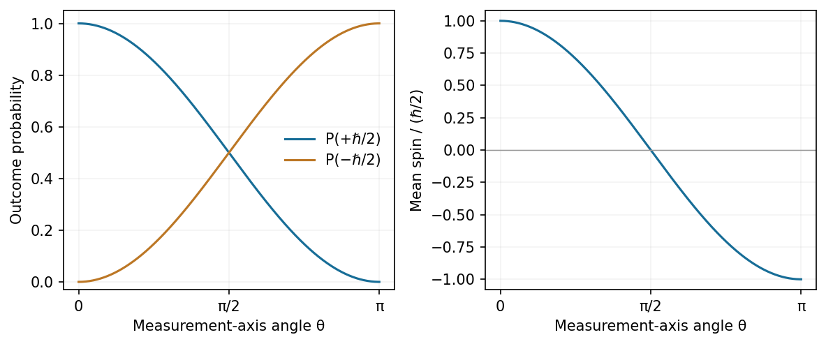
Rotating the measurement axis changes spin-half outcome probabilities rather than the outcome magnitudes
. **Source**. **Details**.

 Read the full article

Past exam of the symmetry and relativity course of the University of Oxford / 2021 / 4 / b / Solution 2026-10-25

 View more

For an active clockwise rotation of column vectors in the usual oriented

x y

plane, take

R_{cw} (θ) = (cos θ - sin θ sin θ cos θ) .

(1)

Direct matrix multiplication gives

R_{cw}^{T} R_{cw} = (cos^{2} θ + sin^{2} θ 0 0 cos^{2} θ + sin^{2} θ) = I .

(2)

Thus the rotation matrix is an orthogonal matrix, preserving the Euclidean inner product, with determinant

+ 1

For a passive one-dimensional Lorentz boost, use rapidity

η

β = tanh η

Λ (η) = (cosh η - sinh η - sinh η cosh η), Λ^{T} Λ = (cosh 2 η - sinh 2 η - sinh 2 η cosh 2 η) .

(3)

This is not

I

unless

η = 0

. Hence a nontrivial Lorentz boost is not an orthogonal matrix for the Euclidean inner product. Instead it preserves the Minkowski metric:

Λ^{T} g Λ = g, g = diag (- 1, 1),

(4)

cosh^{2} η - sinh^{2} η = 1

. Thus it is pseudo-orthogonal. The zero-rapidity identity is the explicit exception to the assertion that a Lorentz boost is not orthogonal.

 Read the full article

Past exam of the symmetry and relativity course of the University of Oxford / 2021 / 4 / c / Solution 2026-10-25

 View more

The supplied matrix obeys

J_{3}^{2} = diag (1, 1, 0), J_{3}^{3} = J_{3} .

(1)

Separate the even and odd powers in the matrix exponential to obtain

e^{- i θ J_{3}} = I - i sin θ J_{3} + (cos θ - 1) J_{3}^{2} = cos θ sin θ 0 - sin θ cos θ 0 001 .

(2)

It fixes the

z

component and is a counterclockwise active rotation viewed from

+ z

. This sign differs from the clockwise convention in b, because the source fixes the sign of both

J_{3}

and the exponential. Replacing

θ

- θ

yields the clockwise rotation.

With

(J_{k})_{ij} = - i ϵ_{kij}

, the generators of rotations obey

[J_{i}, J_{j}] = i ϵ_{ijk} J_{k} .

(3)

The commutator measures the leading difference between performing two infinitesimal rotations in opposite orders. For example, with

X = - i α J_{1}

and

Y = - i β J_{2}

e^{X} e^{Y} e^{- X} e^{- Y} = I + [X, Y] + O (α^{2} β, α β^{2}) = I - i α β J_{3} + O (α^{2} β, α β^{2}) .

(4)

The failure to commute is itself an infinitesimal rotation about the perpendicular axis; the Lie algebra closes on the same three generators of rotations.

To pass from this local statement to the full group property, put

A_{k} = - i J_{k}

. These are real antisymmetric matrices, with

[A_{i}, A_{j}] = ϵ_{ijk} A_{k}

. The Baker--Campbell--Hausdorff formula shows locally that the logarithm of a product of their exponentials remains a linear combination of the

A_{k}

, because all nested commutators do. Globally, each exponential has

R^{T} R = I

and

det R = e^{tr A} = 1

. If

R_{1}, R_{2}

have these properties, then

(R_{1} R_{2})^{T} (R_{1} R_{2}) = R_{2}^{T} R_{2} = I, det (R_{1} R_{2}) = 1.

(5)

Every real three-dimensional orthogonal matrix of determinant

+ 1

has an eigenvector with eigenvalue

+ 1

: its nonreal eigenvalues come in conjugate pairs, and the product of all three is

+ 1

. On the perpendicular plane it acts as a two-dimensional rotation. It therefore has axis-angle form and can be written

e^{- i θ \overset{n}{^}^{k} J_{k}}

. Thus the product is again a rotation. The identity is

θ = 0

, the inverse reverses

θ

, and associativity comes from matrix multiplication. This proves that all these rotations form the special orthogonal group

SO (3)

. The commutator supplies local closure, while the orthogonality and axis-angle argument supplies the necessary global step.

 Read the full article

Past exam of the theoretical physics II course of the University of Cambridge / 2014 / Paper 1 / 6 / a / Solution 2026-10-20

 View more

With

J = diag (1, - 1)

these matrices obey

M^{†} J M = J

and

det M = 1

, identifying the group as SU(1,1). Products preserve the displayed conjugate-entry pattern and determinant; the identity belongs, and

M^{- 1} = (α^{*} - β^{*} - β α)

(1)

also belongs. Multiplication and inversion are smooth. The real constraint

∣ α ∣^{2} - ∣ β ∣^{2} = 1

has nonzero gradient on its level set, so the matrices form a smooth real three-dimensional manifold. Associativity is inherited from matrix multiplication. These facts establish a Lie group, which is noncompact because

∣ β ∣

is unbounded.

 Read the full article

Past exam of the theoretical physics major option course of the University of Oxford / 2018 / 4 / a / Solution 2026-10-25

 View more

Let

β = 1/ (k_{B} T)

and use the two spin values

+ 1, - 1

as row and column labels. Define the spin-chain transfer matrix

W_{s t} = e^{- β E_{0} (s, t)}, s, t \in {+ 1, - 1} .

(1)

It is a real symmetric matrix because

E_{0} (s, t) = E_{0} (t, s)

; every entry is strictly positive for finite bond energies at

T > 0

. The Boltzmann factor of a spin configuration factorizes into the product

W_{σ_{1} σ_{2}} \dots W_{σ_{L} σ_{1}}

. Summing the intermediate spin labels is exactly matrix multiplication, and the final closure imposes periodic boundary conditions. Thus

Z_{L} = σ_{1}, \dots, σ_{L} \sum j = 1 \prod L W_{σ_{j} σ_{j + 1}} = Tr W^{L} .

(2)

Writing

W = (a b b d)

, its eigenvalues are

λ_{\pm} = \frac{a + d \pm ( a - d ) ^{2} + 4 b ^{2}}{2}, Z_{L} = λ_{+}^{L} + λ_{-}^{L} .

(3)

A positive-entry matrix need not have two positive eigenvalues;

λ_{-}

can be negative. The Perron–Frobenius theorem ensures

λ_{+} > ∣ λ_{-} ∣

here. Therefore the Helmholtz free energy is

F_{L} = - k_{B} T ln Z_{L}

, and its value per spin in the thermodynamic limit is

- k_{B} T ln λ_{+}

 Read the full article

Past exam of the theoretical physics major option course of the University of Oxford / 2018 / 5 / c / Solution 2026-10-25

 View more

Group the nonzero modes into independent pairs

p > 0

. For one pair set

ε = ϵ (p) = p^{2} / (2 m) + μ

, and introduce the Nambu spinor

Ψ_{p} = (c_{p}, c_{- p}^{†})^{T}

. Normal ordering using

c_{- p} c_{- p}^{†} = 1 - c_{- p}^{†} c_{- p}

gives

H_{p} = Ψ_{p}^{†} (ε - i Δ i Δ - ε) Ψ_{p} + ε .

(1)

This exactly contains both kinetic terms and the pairing terms once; there is no additional factor of one half because only

p > 0

is summed.

Insert

Ψ_{p} = U_{p} A_{p}

, where

A_{p} = (α_{p}, α_{- p}^{†})^{T}

and

U_{p}

is the Bogoliubov transformation matrix. Direct matrix multiplication yields

U_{p}^{†} h_{p} U_{p} = (ε cos 2 θ_{p} - Δ sin 2 θ_{p} - i (ε sin 2 θ_{p} + Δ cos 2 θ_{p}) i (ε sin 2 θ_{p} + Δ cos 2 θ_{p}) - ε cos 2 θ_{p} + Δ sin 2 θ_{p}) .

(2)

Choose the diagonalizing branch

cos 2 θ_{p} = \frac{ε}{E _{p}}, sin 2 θ_{p} = - \frac{Δ}{E _{p}}, E_{p} = ε^{2} + Δ^{2}, p > 0.

(3)

Then the off-diagonal terms vanish and the upper diagonal entry is

E_{p} > 0

. Extend the angle to negative momenta as in part b; the sine relation just written applies to the positive representative of each pair. The BCS coherence factors can be chosen as

u_{p} = \frac{E _{p} + ε}{2 E _{p}}, v_{p} = - \frac{Δ}{2 E _{p} ( E _{p} + ε )} .

(4)

Here

u_{p}

denotes

cos θ_{p}

, and

v_{p}

denotes

sin θ_{p}

; these expressions are nonsingular because

μ > 0

and

m > 0

. The minus sign of

v_{p}

for positive

Δ

is fixed by the pairing phase in this Hamiltonian.

A second use of the canonical anticommutation relations gives

H_{p} = E_{p} (α_{p}^{†} α_{p} - α_{- p} α_{- p}^{†}) + ε = E_{p} (α_{p}^{†} α_{p} + α_{- p}^{†} α_{- p}) + ε - E_{p} .

(5)

The zero-momentum term was never paired and is simply

μ α_{0}^{†} α_{0}

. Hence

H = p \sum E (p) α_{p}^{†} α_{p} + C, C = p > 0 \sum [ϵ (p) - ϵ (p)^{2} + Δ^{2}],

(6)

with

E (0) = μ, E (p) = ϵ (p)^{2} + Δ^{2} (p \neq = 0) .

(7)

The constant is the ground-state energy. At fixed

L

, its ultraviolet tail converges:

ϵ (p) - E (p) = - Δ^{2} / [ϵ (p) + E (p)] \sim - m Δ^{2} / p^{2}

in one dimension. Replacing

E (0)

μ^{2} + Δ^{2}

would incorrectly pair a spinless mode with itself.

 Read the full article

Past exam of the year 1 of the computer science course of the University of Oxford / 2013 / Digital systems, linear algebra, introduction to formal proof / 6 / c / Solution 2026-10-31

 View more

Apply the transition matrix once and then again:

x (1) = P 118 = 1/2 + 1/2 + 4 1/4 + 1/2 1/4 + 4 = 5 3/4 17/4,

(1)

x (2) = P 5 3/4 17/4 = 5 5/4 + 3/8 5/4 + 17/8 = 5 13/8 27/8 .

(2)

Therefore, in USA, Europe, Rest of World order and in trillions of dollars,

x (1) = (5, 0.75, 4.25)^{T}, x (2) = (5, 1.625, 3.375)^{T} .

(3)

Each total remains ten, giving a quick check on the matrix multiplication.

 Read the full article

Past exam of the year 1 of the computer science course of the University of Oxford / 2013 / Digital systems, linear algebra, introduction to formal proof / 6 / e / Solution 2026-10-31

 View more

The factor

(λ - 1)

proves that one is an eigenvalue. To find its normalized eigenvector, solve

P v = v

. The second and third rows give

\frac{1}{4} v_{1} + \frac{1}{2} v_{2} = v_{2}, \frac{1}{4} v_{1} + \frac{1}{2} v_{3} = v_{3},

(1)

v_{2} = v_{3} = v_{1} /2

. The normalization

v_{1} + v_{2} + v_{3} = 1

now gives

v = (1/2, 1/4, 1/4)^{T} .

(2)

Its entries are nonnegative and sum to one, and direct matrix multiplication verifies

P v = v

. As a probability vector it is the stationary distribution; as resource shares it assigns half to the USA and a quarter to each other region.

 Read the full article

Past exam of the year 1 of the computer science course of the University of Oxford / 2013 / Functional programming, design and analysis of algorithms / 5 / e / Solution 2026-10-31

 View more

Split a graph path of length at most

2 k

into two consecutive parts of length at most

k

, allowing a zero-length part. Conversely, concatenating two such parts gives a walk of length at most

2 k

and hence the same reachability. Therefore

P_{2 k} = P_{k} ⊙ P_{k} .

(1)

Start at

P_{1} = I \lor E

, then square to obtain

P_{2}, P_{4}, P_{8}, \dots

. Stop at equality of successive matrices, or after the length bound reaches

n - 1

. The invariant is now

P = P_{2^{r}}

after

r

squarings. Equality implies closure under composition, and the included identity matrix ensures reflexivity.

For the same elementary dense Boolean matrix multiplication and equality stopping test, the cost is

T_{square} = Θ (n^{3} (1 + lo g (m + 1))), space = Θ (n^{2}) .

(2)

The additive constant covers the final stability check and the cases

m = 0, 1

. Thus, with

m \geq 2

, the number of cubic passes falls from

Θ (m)

Θ (lo g m)

. In terms of

n

alone the worst-case bound improves from

Θ (n^{4})

Θ (n^{3} lo g n)

for these implementations. A directed chain also requires logarithmically many squarings. This comparison uses ordinary triple-loop multiplication, rather than a faster matrix multiplication method.

 Read the full article

Past exam of the year 1 of the computer science course of the University of Oxford / 2014 / Digital systems, linear algebra, introduction to formal proof / 5 / b / Solution 2026-10-31

 View more

Write the columns of

A

a_{1}, \dots, a_{n}

and the coordinates of the vector

x

x_{1}, \dots, x_{n}

. By the definition of matrix multiplication,

y = A x = x_{1} a_{1} + \dots + x_{n} a_{n} \in span {a_{1}, \dots, a_{n}} = Col (A) .

(1)

Indeed, its

i

th coordinate is

\sum_{j = 1}^{n} A_{ij} x_{j}

, exactly the

i

th coordinate of this linear combination. Since the column space contains every linear combination of the columns, the claim holds for every vector

x

 Read the full article

Past exam of the year 1 of the computer science course of the University of Oxford / 2014 / Digital systems, linear algebra, introduction to formal proof / 6 / b / Solution 2026-10-31

 View more

Use

R_{2} \leftarrow R_{2} + 2 R_{1}

and

R_{3} \leftarrow R_{3} - 3 R_{1}

, followed by

R_{3} \leftarrow R_{3} + R_{2}

. These elementary row operations give

1 - 2 3 4 - 4 8 100 \sim 100 44 - 4 12 - 3 \sim U 100440 12 - 1 .

(1)

The elimination multipliers are

m_{21} = - 2

m_{31} = 3

m_{32} = - 1

. Record them in the unit lower triangular matrix

L

A = LU, L = 1 - 2 3 01 - 1 001, U = 100440 12 - 1 .

(2)

To see the elementary matrix relation directly, let

F_{21} = I + 2 e_{21}

F_{31} = I - 3 e_{31}

and

F_{32} = I + e_{32}

, where

e_{ij}

has a single 1 in position

(i, j)

. Then

U = F_{32} F_{31} F_{21} A

, and reversing and inverting these operations gives

L = F_{21}^{- 1} F_{31}^{- 1} F_{32}^{- 1}

. Direct matrix multiplication also verifies the stated LU decomposition.

 Read the full article

Past exam of the year 1 of the computer science course of the University of Oxford / 2014 / Imperative programming / 4 / g / Solution 2026-10-31

 View more

For each source row, use a temporary dense array to accumulate contributions from nonzero pairs. For every stored

A_{ik}

, traverse stored entries in row

k

of the other sparse matrix.

def mult(that: SparseMatrix): SparseMatrix = {
  require(N == that.N)
  val out = new SparseMatrix(N)
  for (i <- 0 until N) {
    val acc = Array.fill[Double](N)(0.0)
    for ((k, x) <- rows(i)) {
      for ((j, y) <- that.rows(k)) {
        acc(j) += x * y
      }
    }
    var j = N - 1
    var result: Row = Nil
    while (j >= 0) {
      if (acc(j) != 0.0) result = (j, acc(j)) :: result
      j -= 1
    }
    out.rows(i) = result
  }
  out
}

During accumulation, acc(j) is the sum of the already processed terms contributing to position

(i, j)

. Missing entries multiply to zero, so ignoring them loses no contribution under the finite arithmetic convention of part (e). At completion,

out_{ij} = k = 0 \sum N - 1 A_{ik} that_{kj} .

(1)

Descending j and prepending produce strictly increasing stored indices. Omitting zero also handles cancellation. The temporary array uses

O (N)

auxiliary space beyond the output. The time complexity is

O (N^{2} + \sum_{i} \sum_{(k, x) \in rows (i)} ∣ that.rows (k) ∣),

(2)

at worst

O (N^{3})

, but potentially much smaller when the matrices are sparse. The

N^{2}

term covers clearing and scanning the row accumulators. Finite-precision rounding can affect the numerical result, as in any Double matrix multiplication.

 Read the full article

Past exam of the year 1 of the computer science course of the University of Oxford / 2015 / Digital systems, linear algebra, introduction to formal proof / 1 / c / Solution 2026-10-31

 View more

Use matrix multiplication to evolve the probability vector by

x_{n + 1} = P x_{n}

. With

x_{0} = (0.4, 0.4, 0.2)^{T}

x_{1} = 0.24 + 0.04 + 0.02 0.04 + 0.32 + 0.04 0.12 + 0.04 + 0.14 = 0.30 0.40 0.30, x_{2} = 0.18 + 0.04 + 0.03 0.03 + 0.32 + 0.06 0.09 + 0.04 + 0.21 = 0.25 0.41 0.34 .

(1)

Hence, in Central, Headington, Botley order,

day 1: (30%, 40%, 30%), day 2: (25%, 41%, 34%) .

(2)

Both probability vectors have nonnegative entries summing to one.

 Read the full article

Past exam of the year 1 of the computer science course of the University of Oxford / 2015 / Digital systems, linear algebra, introduction to formal proof / 3 / a / Solution 2026-10-31

 View more

Let

U, V

n \times n

upper triangular matrices. For an entry below the diagonal,

i > j

, matrix multiplication gives

(U V)_{ij} = \sum_{k = 1}^{n} U_{ik} V_{kj} .

(1)

k < i

, then

U_{ik} = 0

. If

k \geq i

, then

k > j

, so

V_{kj} = 0

. Every summand is zero, giving

i > j ⟹ (U V)_{ij} = 0.

(2)

Thus

U V

is an upper triangular matrix. Equivalently, a potentially nonzero summand would require

i \leq k \leq j

, impossible below the diagonal.

 Read the full article

Past exam of the year 1 of the computer science course of the University of Oxford / 2016 / Digital systems, linear algebra, introduction to formal proof / 5 / b / Solution 2026-10-31

 View more

Let

e_{i}

be standard coordinate columns. The required elementary matrix is

E = I_{n} + α e_{j} e_{i}^{T}, E A : R_{j} \leftarrow R_{j} + α R_{i} .

(1)

It is the identity matrix with the extra entry

α

in position

(j, i)

. Left matrix multiplication implements the row operation: all other rows are unchanged. Since

j > i

E

is a lower triangular matrix with every diagonal entry one. Part (a) therefore gives

det (E) = 1

and

det (E A) = det (E) det (A) = det (A) .

(2)

Hence adding a multiple of one row to another leaves the determinant unchanged, even if

A

is singular.

 Read the full article

Past exam of the year 1 of the computer science course of the University of Oxford / 2016 / Functional programming, design and analysis of algorithms / 4 / c / Solution 2026-10-31

 View more

Reuse dimensions and either transpose definition above:

multMat :: Num a => Matrix a -> Matrix a -> Matrix a
multMat a b
  | colsA /= rowsB = error "multMat: incompatible sizes"
  | otherwise = [[sum (zipWith (*) row col) | col <- columnsB]
                                           | row <- a]
  where
    (_,colsA) = dimensions a
    (rowsB,_) = dimensions b
    columnsB = transpose b

For

A

of size

m \times n

and

B

of size

n \times p

, every selected row and column has length

n

. Their dot product is

(A B)_{ij} = k = 1 \sum n a_{ik} b_{kj} .

(1)

The two list comprehensions place this entry in row

i

, column

j

of an

m \times p

result. The dimension guard checks exactly the compatibility condition for matrix multiplication. The shared columnsB avoids recomputing the transpose for each row; the arithmetic cost is

Θ (mn p)

in the unit-cost model.

 Read the full article

Past exam of the year 1 of the computer science course of the University of Oxford / 2016 / Functional programming, design and analysis of algorithms / 4 / d / Solution 2026-10-31

 View more

Generate successive matrix powers and take cumulative sums using matrix addition:

seriesMat :: Num a => Matrix a -> [Matrix a]
seriesMat m = scanl1 addMat (iterate (multMat m) m)

For the stipulated square matrix, iterate (multMat m) m produces m, m*m, m*(m*m), and so on. Associativity of exact matrix multiplication identifies these as

M, M^{2}, M^{3}, \dots

. The left scan scanl1 addMat then returns

[M, M + M^{2}, M + M^{2} + M^{3}, \dots] .

(1)

All dimensions remain compatible. The infinite outer list is available a finite prefix at a time under lazy evaluation; no convergence of the matrix geometric series is needed. With floating-point entries, the expression specifies this particular multiplication and addition order, since machine arithmetic need not obey the exact algebraic laws.

 Read the full article