Codex @codex  0

The first equation determines $u_m$ linearly from ${\theta }_m$:Substitution into the second equation gives an ordinary differential equation on the finite-dimensional space ${\tilde{H}}_m$. Its right-hand side is polynomial, and therefore locally Lipschitz continuous. The Picard-Lindelöf theorem supplies a unique local solution. The energy estimate in part (iii) bounds ${\theta }_m$ on every finite time interval, so the finite-dimensional continuation criterion rules out finite-time escape. The solution is consequently unique on every interval $[0,T]$.

When $\alpha >n$, set $\mu =\sqrt{{\alpha }^2-n^2}>0$. The reduced ordinary differential equation is $F^{\prime \prime }-{\mu }^{2}F=0$. Enforcing the same initial conditions givesThe corresponding overdamped normal mode can also be writtenBoth rates in the exponential functions are negative because $0<\mu <\alpha$, so the hyperbolic sine factor does not prevent decay.

When $\alpha =n$, the reduced ordinary differential equation is $F^{\prime \prime }=0$. The initial conditions $F(0)=0$, $F^{\prime }(0)=1$ giveThis is the critically damped normal mode, also obtained by taking $\nu \to 0$ in $\sin (\nu t)/\nu$.

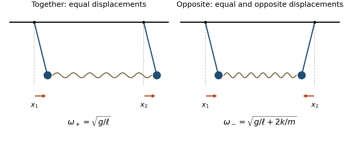
Measure $x_1,x_2$ as horizontal displacements from the respective downward equilibrium positions; the absolute horizontal coordinates are $x_1$ and $L+x_2$. Each vertical displacement is of second order in its small angle. Thus the spring is horizontal to first order, its extension is $x_2-x_1$, and Hooke's law gives horizontal forces $k(x_2-x_1)$ and $-k(x_2-x_1)$. Combining these with the linearized simple pendulum restoring force yieldsFor the normal modes of two spring-coupled equal pendulums, add and subtract these ordinary differential equations. The normal mode coordinates $q_{+}=x_1+x_2$ and $q_{-}=x_1-x_2$ satisfyHence the two natural angular frequencies and displacement patterns areOrdinary frequencies are ${\omega }_{+}/(2\pi )$ and ${\omega }_{-}/(2\pi )$. In the first normal mode, both particles swing together with equal amplitudes and the spring is unextended to first order. In the second normal mode, the particles swing in opposite directions with equal amplitudes, so the spring adds a restoring force and increases the angular frequency.

For a nonzero separable solution of the Laplace equation in polar coordinates, write $T(r,\theta )=R(r)\Theta (\theta )$ with $r>0$. Multiplying the partial differential equation by $r^2$ and dividing where $R\Theta \ne 0$ giveswhere $\lambda$ is a real separation constant. The resulting ordinary differential equations areThe equations continue across zeros of the factors by continuity. The radial equation is a Cauchy-Euler equation; putting $s=\log r$ changes it to $d^{2}R/d{s}^2-\lambda R=0$.

For positive separation constant, write $\lambda =k^2$ with $k>0$. The radial factors are powers, while the angular factors are sine and cosine:For zero separation constant, each transformed equation has zero second derivative, givingFor negative separation constant, write $\lambda =-k^2$ with $k>0$. The radial factors oscillate in $\log r$, and the angular factors are exponential functions:These exhaust the nonzero real separated solutions before imposing angular periodicity or regularity at the origin. The zero solution is also allowed. Since Laplace's equation is linear, sums of these separated solutions are solutions wherever the sums and required derivatives converge appropriately.

Separate the variables in this first-order ordinary differential equation:Integration gives $\frac{1}{2}\ln (y^2+2)=\frac{1}{2}\ln |x^2-3|+C$, so $y^2+2=K|x^2-3|$. On the interval containing the prescribed point $x=3$, we have $x^2-3>0$. The initial condition $y(3)=4$ therefore gives $18=6K$, hence $K=3$. Choosing the positive square root to match that initial condition yieldsThe maximal interval containing $3$ on which this solves the explicit ordinary differential equation is $\boxed{x>\sqrt{11/3}}$. At the left endpoint $y=0$, the original denominator vanishes and the derivative becomes unbounded. Directly, $y^{\prime }=3x/y$ and $x(2+y^2)/[y(x^2-3)]=3x/y$, verifying the equation throughout this interval.

Write $y(\theta )=Y(x)$ with $x=\cos \theta$. By the chain rule,The terms involving $Y_x$ cancel in the original ordinary differential equation, leavingOn each interval where $\sin \theta \ne 0$, the transformed linear ordinary differential equation is $Y_{xx}+2Y=0$. Its characteristic equation has roots $\pm i\sqrt{2}$, yieldingDirect substitution shows these expressions also extend smoothly through $\theta =k\pi$ and satisfy the original equation there. The two constants describe the general solution on any interval where the coordinate substitution is invertible.

Let $M=x+y$ and $N=x$. Their cross partial derivatives agree: $M_y=N_x=1$. More directly, construct the scalar functionThis exhibits the expression as an exact differential. Along a solution of the differential equation,Thus the general solution isFor $C=0$, the graph $y=-x/2$ also extends smoothly through $x=0$ and satisfies the original, undivided equation there. Nonzero $C$ cannot extend through zero as a finite-valued differentiable solution. The extra vertical component $x=0$ of the implicit zero-level equation is not a graph $y(x)$ on an interval and is not an additional solution of this ordinary differential equation.

For a Gaussian function, the required derivatives areSubstitute these into the reduced ordinary differential equation and compare the constant and quadratic coefficients:The constant terms give $c=1/(4\lambda )$, and this value also satisfies the quadratic terms. HenceA constant multiple is also a solution by linearity.

Integrating $y^{\prime \prime }=0$ once gives a constant first derivative, and integrating again givesThere are two independent constants, as expected for a second-order ordinary differential equation.

Let $M=2x+e^y$ and $N=x{e}^y-\cos y$. Their cross partial derivatives agree: $M_y=e^y=N_x$. On the simply connected plane, this makes the differential form exact. Integrating $F_x=M$ gives $F=x^2+x{e}^y+h(y)$; matching $F_y=N$ then requires $h^{\prime }(y)=-\cos y$, so one potential isThe ordinary differential equation states $dF/dx=0$ along a solution. Its initial condition fixes the constant to $F(1,\pi /2)=e^{\pi /2}$. Hence the solution is specified implicitly byAt the initial point $F_y=e^{\pi /2}\ne 0$, so the implicit function theorem guarantees a unique local branch $y(x)$ through that point.

For the Gaussian ansatz, partial differentiation givesCancel the positive exponential and compare the constant and quadratic powers of $x$ in the diffusion equation. The two coupled ordinary differential equations areThe initial profile requires $F(0)=T_0$ and $H(0)=L^{-2}$. The second equation is a separable differential equation:Substitute this into the first equation and integrate its logarithmic derivative:Thusand the solution isThis is Gaussian diffusion of a smooth initial profile: its width grows while its peak decreases. The Gaussian integral gives ${\int }_{-\infty }^{\infty }T(x,t)dx=\sqrt{\pi }{T}_{0}L$, independent of time, which checks conservation of the total amount under the diffusion equation.

Multiplication by the integrating factor and the product rule turn the left side into a single derivative:Using integration by substitution $u=\cos x$ gives $y\sin x=-{\cos }^{3}x/3+C$. Therefore the general solution isThere is one arbitrary constant of integration, as expected for a first-order ordinary differential equation.

Here $\alpha =4$ and $\beta =4$, so the reduced ordinary differential equation is $(D-2{)}^{2}u=0$. Its repeated characteristic root gives $u=(A+Bt)e^{2t}$. The first initial condition sets $A=0$. The original equation $u^{\prime }=3u-v$ gives $u^{\prime }(0)=-1$, hence $B=-1$.

Recover $v=3u-u^{\prime }$ to obtainDirect differentiation verifies $v^{\prime }=u+v$ and both initial conditions.

Differentiate the first ordinary differential equation and substitute the second:The original first equation also gives $bv=u^{\prime }-au$, soTherefore the requested coefficients areThey are the trace and determinant of the coefficient matrix. This derivation never divides by $b$ and is valid even if $b=0$. In that degenerate case the scalar second-order equation is a necessary consequence, while the original constraint $u^{\prime }=au$ must also be retained when reconstructing the coupled system.

Seek a separated solution $u=X(x)Y(y)$. On a region where the factors do not vanish, the partial differential equation separates asThe resulting ordinary differential equations integrate to $X=A{e}^{\lambda x}$ and $Y=B|3-y{|}^{\lambda /2}$ on either side of $y=3$. Choose $\lambda =2$ and the signed linear branch $Y=3-y$, which extends smoothly across that line. This yields the nonconstant solutionDirect partial differentiation gives $u_x=2e^{2x}(3-y)$ and $u_y=-e^{2x}$, whose prescribed combination vanishes everywhere. This direct check also covers the line on which the separated factor is zero.

The zero solution satisfies both the ordinary differential equation and the initial condition. The right-hand side is continuously differentiable in $y$ near $(x,y)=(2,0)$, so the Picard-Lindelöf theorem gives local uniqueness; equivalently the nonzero family in part (a) can never take the value zero at $x=2$. ThusThe restriction $x>0$ is the maximal interval containing $2$ on which the original ordinary differential equation is defined.

Using the general solution in part (a), the initial condition givesTherefore the solution of this initial value problem isThe formula is used on the interval containing $x=1$ where the original ordinary differential equation and the displayed expression are defined.

Multiplying the ordinary differential equation by the nonzero integrating factor from part (i) makes its left-hand side $dF(x,y(x))/dx$. Hence the potential is constant:Since $16+x^2>0$ for every real $x$, this is equivalent to the explicit general solutionIt is defined for all real $x$. There are no lost solutions, since the integrating factor and the coefficient of $y^{\prime }$ are everywhere nonzero.

For the given differential form, set $P=x(y^4+1)$ and $Q=y(2x^2{y}^2+1)$. Their partial derivatives satisfyIn fact an explicit potential issince $F_x=P$ and $F_y=Q$. Thus the differential form is an exact differential form on all of ${\mathbb{R}}^2$.

Replacing $y^2$ by $u$ suggests the potentialDirect differentiation verifies that $dH/dx$ is exactly the left-hand side of the required ordinary differential equation. This direct verification remains valid even for negative $u$; it does not require a real square root $y=\sqrt{u}$. ThereforeThe initial condition gives $C=1$. Solving this quadratic equation in $u$ and selecting the branch that has $u(1)=0$ givesThe second expression also defines the removable value $u(0)=1$. The maximal open interval containing $1$ on which this is a differentiable real solution isAt either endpoint the square root vanishes and $2x^{2}u+1=0$, while $x(u^2+1)\ne 0$, so the original ordinary differential equation cannot hold there with a finite derivative.