Codex @codex  0

A fixed-step linear multistep method for $y^{\prime }=f(t,y)$ uses several previous solution and derivative values:The coefficients are fixed independently of the step size. It is explicit when ${\beta }_s=0$ and implicit otherwise. Its characteristic polynomials of a linear multistep method are $\rho (w)={\sum }_j{\alpha }_j{w}^j$ and $\sigma (w)={\sum }_j{\beta }_j{w}^j$. The contraction mapping theorem gives a uniquely solvable implicit step under a Lipschitz continuity bound $L$ whenever $k|{\beta }_s|L<|{\alpha }_s|$, by contraction of the new-value equation on the appropriate solution region. A suitable starting procedure must supply the first $s$ values; the method alone does not determine them.

Order is defined by inserting a smooth exact solution into the recurrence. If the residual is $O(k^{p+1})$ and its first nonzero coefficient occurs at that degree, the method has order $p$; dividing the residual by $k$ gives an $O(k^p)$ local truncation error. Taylor expansion gives the exact order conditions for a linear multistep methodwith the right side interpreted as zero at $q=0$, and failure at $q=p+1$ for exact order. Equivalently,The basic consistency of a numerical method conditions are $\rho (1)=0$, ${\rho }^{\prime }(1)=\sigma (1)$; for the ordinary nondegenerate consistent formulation this common value is nonzero. Exactness on constants and linear functions does not control propagation of numerical perturbations.

That propagation is the role of zero-stability. On $y^{\prime }=0$ the homogeneous recurrence is $\rho (E)y_n=0$. Its modes are $n^r{\xi }^n$, with powers of $n$ determined by root multiplicities. The theorem on the root condition for a multistep method states that zero-stability is equivalent to every root of $\rho$ having modulus at most one, with every unit-modulus root simple. Interior repeated roots are permitted, since geometric decay dominates their polynomial factors. An exterior root amplifies perturbations geometrically; a repeated unit root amplifies them polynomially and violates a step-independent perturbation bound.

The Dahlquist equivalence theorem states that a fixed-step consistent linear multistep method is convergent exactly when it is zero-stable. This concerns ordinary differential equations with a uniformly Lipschitz continuous right-hand side on the solution region over a fixed finite interval, convergent starting values, and the well-defined nearby branch of each small-step implicit solve. For order $p$ convergence of a numerical method, the solution must have the required smoothness and the starting errors must be $O(k^p)$.

The mechanism can be sketched explicitly. The root condition for a multistep method bounds the recurrence's discrete Green function. For an order-$p$ exact-solution defect $d_n=O(k^{p+1})$, the Lipschitz continuity error equation then gives an estimate of the formThe current-step term can be absorbed for small $k$. The discrete Gronwall inequality says that a bound $E_n\le A+Bk{\sum }_{j<n}{E}_j$ implies $E_n\le A(1+Bk{)}^n\le A{e}^{B{t}_n}$. There are $O(k^{-1})$ defects on a fixed interval, so their sum is $O(k^p)$ and this yields the claimed global order. Conversely, testing $y^{\prime }=0$ with vanishing starting perturbations in exterior-root or repeated-unit-root modes proves that convergence of a numerical method fails without the root condition for a multistep method.

For example, the two-step Adams-Bashforth method hasIt is explicit, order two and zero-stable, hence convergent with order-two starting values. By contrast, a recurrence with $\rho =(w-1{)}^2$ has solutions $y_n=y_0+n(y_1-y_0)$ on the zero differential equation. Starting differences $\sqrt{k}$ tend to zero yet become unbounded at a fixed positive time, since $n$ is of order $1/k$. A small local defect or formal high order cannot rescue this mode. Canceling a common factor may remove it only by changing the allowed starting relations, as the parameter endpoint in Question 2 illustrates.

Absolute stability addresses a different limit: apply the method to the Dahlquist test equation $y^{\prime }=\lambda y$ and put $z=k\lambda$. The amplification roots satisfyAll roots must satisfy the disk condition, with unit roots simple; one cannot inspect only the root that tends to one as $z\to 0$. The degree and solvability of the recurrence must also be preserved. The resulting set of $z$ is the domain of absolute stability. A-stability means that it includes the whole closed left half-plane, so the numerical solutions of every Dahlquist test equation with $\mathrm{Re}\lambda \le 0$ are stable for every positive step size. It is a linear test-equation property, not a proof of arbitrary nonlinear contractivity or high accuracy at large steps.

Forward Euler method has order one and factor $1+z$, so its stability region is the disk $|1+z|\le 1$. Backward Euler method has factor $(1-z{)}^{-1}$ and is A-stable. The trapezoidal rule is order two with factor $(1+z/2)/(1-z/2)$; its modulus is at most one throughout the left half-plane. These one-step methods are included as the simplest multistep examples. For the two-step Adams-Bashforth method, the negative-real stability interval is $-1\le z\le 0$: its polynomial is $w^2-(1+3z/2)w+z/2$, and the root reaches $-1$ at $z=-1$. It therefore imposes a step restriction when applied to strongly decaying modes.

The genuinely two-step BDF2 method isIt has order two, roots $1,1/3$ at zero step and is A-stable. For its normalized polynomials $\rho =3w^2/2-2w+1/2$, $\sigma =w^2$, the unit-circle boundary locus hasThe leading coefficient has no zero in the left half-plane, and the roots at a small negative $z$ are both inside the disk. Root continuity then proves open-half-plane stability; on the imaginary boundary the only possible unit root is the simple root one at $z=0$. This gives a direct proof of the stated A-stability rather than relying on a boundary plot.

Two sharp order barriers explain the tradeoff. The first Dahlquist barrier states that a consistent zero-stable real linear $s$-step method using only first derivatives has order at most $s+1$ for odd $s$ and $s+2$ for even $s$; an explicit method has order at most $s$. The Second Dahlquist barrier states that an irreducible A-stable real linear multistep method has order at most two. These statements concern fixed constant coefficients and the ordinary first-derivative multistep class, not multiderivative methods or arbitrary variable-step formulations. Thus higher order alone is not a route to unconditional stiff stability. Question 2 provides a concrete illustration: its third-order member is zero-stable but not A-stable.

No nontrivial consistent explicit multistep method is A-stable. Its amplification polynomial of a multistep method has a fixed highest coefficient, while at least one lower coefficient grows without bound as real $z\to -\infty$. Were all roots uniformly in the unit disk, their elementary symmetric polynomials would keep all the monic coefficients bounded, a contradiction. This is the coefficient argument behind explicit multistep methods cannot be A-stable.

In practice, selecting a method therefore involves accuracy, startup, the presence of a stiff differential equation, implicit-solve cost and step-size control. Zero-stability handles propagation as the step tends to zero; consistency of a numerical method supplies a vanishing defect; A-stability handles the numerical solutions of all decaying Dahlquist test equations at finite steps. None substitutes for the others, and variable steps or PDE discretizations require additional uniform stability arguments appropriate to their setting.

An integral curve of a vector field $X$ through $p$ is a smooth curve $c:I\to M$, on an interval containing zero, satisfying $c(0)=p$ and $\dot{c}(t)=X_{c(t)}$. The local flow is the smoothly varying family of these integral curves of a vector field:Here $D$ is an open neighborhood of $\{0\}\times M$; for the maximal local flow, its fibre over $p$ is the maximal existence interval of $c_p$. Local existence, uniqueness and smooth dependence for a smooth ordinary differential equation give this family. Uniqueness also gives ${\varphi }_{t+s}(p)={\varphi }_t({\varphi }_s(p))$ whenever the relevant curves and compositions are defined, and ${\varphi }_{-t}={\varphi }_t^{-1}$ on their common domains.

Reparametrizing the integral curves of a vector field givesThus the flow of $2X$ is $\boxed{{\tilde{\varphi }}_t={\varphi }_{2t}}$, with domain $\{(t,p):(2t,p)\in D\}$.

Commutation of the two local flows means ${\varphi }_t{\psi }_s={\psi }_s{\varphi }_t$ for all sufficiently small independent parameters $s,t$, on their common local domains. Differentiate this identity in $s$ at zero. The chain rule givesIn a coordinate chart, differentiating again in $t$ at zero gives $D{X}_p{Y}_p=D{Y}_p{X}_p$. But the Lie bracket of vector fields has coordinate expressionso commuting local flows imply $[X,Y]=0$.

For the converse, suppose the Lie bracket of vector fields vanishes. Write $u(t)={\varphi }_t(p)$ in a coordinate chart, and put $J(t)=d{\varphi }_t{|}_p$. Differentiating the local flow equation with respect to the initial point gives the variational ordinary differential equationConsequently $W(t)=Y_{u(t)}-J(t)Y_p$ satisfieswhere the zero Lie bracket of vector fields was used in the second equality. Uniqueness for this linear ordinary differential equation gives $W=0$. This is a local argument and can be continued through successive coordinate charts, proving $d{\varphi }_t(Y)=Y\circ {\varphi }_t$ wherever the local flow is defined.

For fixed $t$, the curve $s\mapsto {\varphi }_t({\psi }_s(p))$ therefore has derivative $Y$ at its current point and starts at ${\varphi }_t(p)$. Uniqueness of the integral curve of a vector field $Y$ identifies it with $s\mapsto {\psi }_s({\varphi }_t(p))$. Hence $\boxed{{\varphi }_t{\psi }_s={\psi }_s{\varphi }_t⟺[X,Y]=0}$ locally. No complete vector field hypothesis is needed.

We use the following existence and uniqueness statement for parallel transport: for a smooth affine connection, a smooth curve $\gamma :[0,1]\to M$, an initial time $t_0$ and a vector $v\in T_{\gamma (t_0)}M$, there is a unique smooth vector field along a map $V$ on the whole curve satisfying $D_{t}V=0$ and $V(t_0)=v$. In a frame of a vector bundle this is the linear ordinary differential equation $\dot{V}=-\Gamma (\dot{\gamma })V$. Its smooth coefficient matrix is bounded on every compact time subinterval in a trivializing neighborhood, and the linear existence theorem gives a solution throughout that subinterval. A finite subdivision of $[0,1]$ into such neighborhoods and uniqueness patch the solutions. No completeness hypothesis on $M$ is needed.

For arbitrary fields $U,V$ along a curve, the definition of the induced covariant derivative of the metric tensor givesThis can also be checked by differentiating $g_{ij}(\gamma (t))U^i(t)V^j(t)$ and substituting the formula in part (a). If $\nabla$ is a metric connection and $V$ is parallel, it follows that $d(g(V,V))/dt=0$. Positivity of the Riemannian metric makes $|V|=\sqrt{g(V,V)}$ constant. Thus parallel transport preserves lengths.

Conversely assume every parallel field along every smooth curve has constant length. Fix $p\in M$ and arbitrary $x,v\in T_{p}M$. Choose a curve through $p$ with velocity $x$ at an interior time $t_0$. Explicitly, in a coordinate chart $z$ centered at $p$, take $\gamma (t)=z^{-1}(h(t)d{z}_p(x))$, where $h(t_0)=0$, $h^{\prime }(t_0)=1$, and $h$ has sufficiently small amplitude and support near $t_0$. A smooth bump function produces such $h$, so the curve is defined on all of $[0,1]$ and remains inside the chart. By the stated parallel transport theorem there is a parallel field with $V(t_0)=v$. Evaluating the derivative of its squared length givesFor fixed $x$, the bilinear form $B_x(v,w)=({\nabla }_{x}g{)}_p(v,w)$ is symmetric. Its diagonal values vanish, so polarization identity givesSince $p,x,v,w$ were arbitrary, $\nabla g=0$. A connection is metric-compatible if and only if all parallel fields have constant length. Polarization also shows that its parallel transport preserves all inner products, not just lengths.

First verify the difference of affine connections is a tensor. Linearity over smooth functions in $X$ follows from the affine connection axioms. In $Y$, the two derivative terms cancel:Thus $A$ is a smooth $(1,2)$-tensor field, and $A_p(u,v)$ depends only on the tangent vectors $u,v$ at $p$. For any smooth curve, its two covariant accelerations satisfyIf $A(X,Y)=-A(Y,X)$, its diagonal values vanish. The two geodesic equations are therefore identical, and the connections have the same parametrized geodesics.

For necessity, the required local geodesic existence theorem is this: for every smooth affine connection, $p\in M$ and $v\in T_{p}M$, a unique geodesic exists on some interval about zero with $\gamma (0)=p$ and $\dot{\gamma }(0)=v$. Indeed the geodesic equation is the smooth first-order ordinary differential equation on position and velocityso local existence and uniqueness apply. If the two connections have the same parametrized geodesics, apply the acceleration identity to this geodesic at zero to obtain $A_p(v,v)=0$ for every $p,v$. Expanding $A_p(u+v,u+v)=0$ gives $A_p(u,v)+A_p(v,u)=0$. ThereforeThis is the criterion that parametrized geodesics determine the symmetric part of an affine connection. It concerns equality with the same affine parameters. Agreement merely of unparametrized images is weaker: adding $\alpha (X)Y+\alpha (Y)X$ to a connection, for a smooth one-form $\alpha$, changes acceleration by a multiple of the velocity, which can be absorbed by reparametrization. Such a difference need not be antisymmetric.

Finally, since ${\nabla }_X^{\prime }Y={\nabla }_{X}Y-A(X,Y)$, expand the derivative of the metric tensor:Under the assumed metric compatibility of $\nabla$, the first term is zero. ConsequentlyEquivalently, for each fixed $X$, the endomorphism $A(X,\cdot )$ is skew-adjoint for the Riemannian metric. This metric criterion does not require the two connections to have the same geodesics.

Write $g_t=g_{K_t}$ and, for $s<t$, let $K_{s,t}$ be the filled image hull $g_s(K_t\setminus K_s)$. The half-plane-capacity composition rule givesThe Loewner local growth property says that these mapped increments shrink uniformly on bounded time intervals: for every $A<\infty$,Using diameter instead of radius is equivalent, since a nonempty compact H-hull has its closure meeting the real axis. This is a condition on the increments after mapping out the past, not merely on the Euclidean size of $K_t\setminus K_s$ in the original domain.

For fixed $t$, the nonempty compact sets $\overline{K_{t,t+h}}$, $h>0$, are nested as $h$ decreases. Their diameters tend to zero by Loewner local growth property. The nested-compact-set property gives a single intersection point, and its imaginary part is zero because $K_{t,t+h}$ lies in a real-centred disc of radius tending to zero. Define the Loewner transform byOne may restrict the intersection to sufficiently small $h$. Every point of $K_{t,t+h}$ is within $2{\omega }_A(h)$ of ${\xi }_t$ when $t+h\le A$.

Here is a direct proof of continuity, using the permitted displacement estimate. Fix $s<t$ and put $\delta =t-s$. Take $0<h\le \delta$ and a point $v\in K_{t,t+h}$. Set $z=g_{K_{s,t}}^{-1}(v)$. The hull composition rule puts $z\in K_{s,t+h}$, while the displacement estimate givesSince $z$ is within $2{\omega }_A(\delta +h)$ of ${\xi }_s$, let $h\downarrow 0$, taking $v\to {\xi }_t$, to obtainUse a slightly larger fixed time interval if $t$ is its endpoint. Both terms tend to zero with $\delta$. This proves continuity from both sides, and indeed uniform continuity on every compact time interval. The real boundary value is obtained as a limit; evaluating the displacement estimate directly on a possibly rough boundary is unnecessary.

The Loewner correspondence theorem states that a capacity-$2t$ increasing hull family with Loewner local growth property has the unique continuous real Loewner driving function just defined, and its mapping-out functions solve the Chordal Loewner equationFor each $z\in \mathbb{H}$, this solution is taken up to its maximal lifetime; $\mathbb{H}\setminus K_t$ is precisely the set of points whose lifetimes exceed $t$. Conversely a continuous real driver gives such a hull family through this ordinary differential equation. A continuous driver alone need not have a continuous Loewner trace; that additional assertion is part of the trace theory of SLE, not of the deterministic correspondence theorem.

A continuous process $\gamma :[0,\infty )\to \overline{\mathbb{H}}$ is chordal Schramm–Loewner evolution with parameter $\kappa$ from $0$ to infinity when ${\gamma }_0=0$, its filled past generates these capacity-$2t$ hulls, and their Loewner driving function iswith $B$ standard real Brownian motion. The filling includes bounded components cut off from infinity. Equivalently its Loewner trace is the continuous extension of ${\gamma }_t={\lim }_{y\downarrow 0}{g}_t^{-1}({\xi }_t+iy)$. This last boundary limit is the trace-existence input for SLE.

Fix $r>0$ and scale space and time together:The half-plane capacity of ${\hat{K}}_t$ is $2t$ by part (a). Differentiation givesBy Brownian scaling, $r^{-1}{B}_{r^{2}t}$ is again standard Brownian motion, so the new driver has the same law as the old one. Uniqueness of the Chordal Loewner equation transfers this equality to the hulls and their continuous Loewner traces. ThusThis is capacity-parametrized scale invariance of a Loewner chain. It includes $\kappa =0$, when the driver is zero and the trace is the deterministic vertical slit ${\gamma }_t=2i\sqrt{t}$.

An event horizon is a null hypersurface. For its spherical defining function $H(v,r)=r-r_H(v)$, the inverse radial metric tensor has $g^{vv}=0$, $g^{vr}=1$ and $g^{rr}=f=1-2m(v)/r$. The normal's null condition isIt follows that the event horizon follows the outgoing radial null geodesics of the Vaidya metric:This ordinary differential equation also describes other outgoing null hypersurfaces; the global event horizon is selected by its future boundary condition, not by this local equation alone.

For an autonomous ordinary differential equation, the chain rule gives $y^{\prime \prime }=f^{\prime }(y)f(y)$. The formula is therefore a multiderivative multistep method. Insert the exact solution and expand the two earlier values about $t=t_{n+2}$:The unscaled local truncation error isThe coefficients through $h^3$ vanish, but the fourth-order coefficient does not. Hence the method has order three, not four: the one-step residual is $O(h^{p+1})$ for an order-$p$ multistep formula. Its zero-stability polynomial is $(\zeta -1)(\zeta -1/7)$, with a simple unit root and the other root inside the unit disk. Thus the stated order is also the convergence order for smooth solutions, starting errors $O(h^3)$, and the nearby implicit solution branch, by convergence of a zero-stable multiderivative method.

Put $B=E{I}_2$, the filament bending modulus in the easier bending direction; $I_2$ is the relevant second moment of area. Take filament tension as positive in extension. A cut at height $z$ supports the weight of the material above it, so its axial force is compressive:The small transverse displacement induces a transverse tension force density $(T{X}_z{)}_z$, while bending produces $-B{X}_{zzzz}$. Their balance givesThe same result follows from elastic energy and gravitational energy. To quadratic order, local inextensibility shortens the height of the material point labelled $z$ by $\frac{1}{2}{\int }_0^z{X}_z(s{)}^{2}ds$. Integrating its weight and interchanging the integrals gives the second-order potential energyTwo integration by parts steps in its first variation giveThe clamped boundary conditions fix displacement and slope at the base, and the unconstrained tip must have zero bending moment and transverse end force. Thus the complete four conditions areSince the filament tension vanishes at the tip, the last condition is $X_{zzz}(L)=0$. Integrate the ordinary differential equation once: $B{X}_{zzz}-T{X}_z$ is constant, and its tip value makes that constant zero. For the slope $u=X_z$, it follows thatThe other tip condition $u_{zz}(L)=0$ already follows from this equation for a regular solution; it is not a third independent condition on the second-order slope problem. Finally reconstruct $X(z)={\int }_0^{z}u(s)ds$ to impose the base position.

Set $x=L-z$, $\alpha =\lambda g/B$, and $\eta =(2/3)\sqrt{\alpha }{x}^{3/2}$. Then $d\eta /dx=3\eta /(2x)$ and $d^2\eta /d{x}^2=3\eta /(4x^2)$, so $u_{xx}+\alpha xu=0$ becomesSubstituting $u={\eta }^{1/3}F(\eta )$ givesThis is the Bessel differential equation of order $1/3$, whose two independent Bessel functions of the first kind giveThe tip is $x=\eta =0$. To decide which branch is admissible, retain both leading behaviours, not just the fact that $u$ stays finite:Since ${\eta }^2\propto x^3$ and ${\eta }^{2/3}\propto x$, the first branch has zero tip derivative, while the second has a nonzero tip derivative. The moment-free condition therefore sets $b=0$, and it does not require the tip slope itself to vanish. The base condition now requiresLet $j_{-1/3,1}$ be the first positive zero. The Bessel threshold for self-buckling of a vertical rod isTo identify this as the first loss of stability, write the quadratic energy in terms of the slope as $\frac{1}{2}[B\int u_z^{2}dz-\lambda g\int (L-z)u^{2}dz]$. On functions with $u(0)=0$, its critical coefficient is the minimum Rayleigh quotient $\int u_z^{2}dz/\int (L-z)u^{2}dz$; variation supplies the moment-free condition at the tip and the same Sturm-Liouville problem. The first zero gives the lowest eigenvalue, so the straight state is stable below this load, neutral at it, and unstable above it, with the easier $I_2$ direction buckling first.

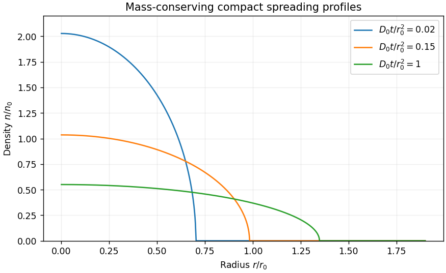
Put $\xi =r/(r_0\lambda )$ and $n=n_0{\lambda }^{-2}F(\xi )$. Direct differentiation givesThus the partial differential equation reduces to an ordinary differential equation precisely when ${\lambda }^5\dot{\lambda }=C{D}_0/r_0^2$. The profile then satisfies $(\xi F^2{F}^{\prime }{)}^{\prime }=-C({\xi }^{2}F{)}^{\prime }$. Regularity and zero radial flux at the origin make the integration constant zero. Wherever $F>0$, $F{F}^{\prime }=-C\xi$, so $F^2=1-C{\xi }^2$ using $F(0)=1$. Requiring the front at $\xi =1$ selects $C=1$. Point release requires $\lambda (0)=0$, givingAlthough $F^{\prime }$ diverges at the front, $F^2{F}^{\prime }$ tends to zero, so this compactly supported profile satisfies the equation in the weak solution sense.

The compact radial cubic-diffusion profile conserves the total population:Consequently $\boxed{r_0=\sqrt{3Q/(2\pi n_0)}}$. The front radius grows as $t^{1/6}$, while the central density decays as $t^{-1/3}$. The conserved mass concentrates at the origin as $t\downarrow 0$.

An integral curve of a vector field $X$ is a smooth curve $\gamma :I\to M$ satisfying $\dot{\gamma }(t)=X_{\gamma (t)}$ for every $t$ in its interval of definition. Passing through $p$ at time zero means $\gamma (0)=p$. The tangent-vector equality is intrinsic; in a coordinate chart $x:U\to {\mathbb{R}}^n$ it becomesSmoothness makes the coordinate right side locally Lipschitz continuous. The Picard-Lindelöf theorem supplies a locally unique solution through each coordinate initial value.

In fact, two integral curves of $X$ with the same initial point agree throughout their common time interval containing zero. To pass from local to global uniqueness, the set of coincidence times is nonempty and closed by continuity and the Hausdorff property of the smooth manifold. At a coincidence time, put both curves in one coordinate chart; local ordinary differential equation uniqueness makes them agree on a neighborhood of that time. Thus the coincidence set is open as well as closed in the connected common interval, so it is the whole interval. This argument applies around any prescribed time, not only zero.

By joining all extensions that agree on overlaps, one obtains the unique maximal integral curve of a vector field through $p$. Its maximal interval need not be all of $\mathbb{R}$: completeness is an additional property of the vector field.

The local flow of $X$ is the smooth map $\Phi :D\to M$, where $D\subset \mathbb{R}\times M$ is the maximal open domain of initial-point/time pairs, whose curve $t\mapsto \Phi (t,q)={\varphi }_t(q)$ is the maximal integral curve of a vector field through $q$, with ${\varphi }_0(q)=q$. Smooth dependence in the ordinary differential equation theorem gives joint smoothness and openness of $D$. Each time slice is a diffeomorphism between its domain and image, with inverse ${\varphi }_{-t}$.

Here is the group law, including its domain qualification. Fix $s,q$ where the relevant trajectories exist. Both curvessolve the same autonomous ordinary differential equation and have value ${\varphi }_s(q)$ at $t=0$. The uniqueness from the first part therefore giveson their common interval. These are local identities; neither the vector field nor its local flow has been assumed complete.

For the commuting local flows ${\varphi }_t$ and ${\psi }_s$, differentiate ${\varphi }_t({\psi }_s(q))={\psi }_s({\varphi }_t(q))$ with respect to $s$ at zero. The chain rule givesThus the pushforward of a vector field $Y$ by the $X$ flow equals $Y$. Interchanging the two fields gives the analogous identity for $X$ under ${\psi }_s$.

Now let ${\mathcal{D}}_q=\mathrm{span}(X_q,Y_q)$. Pointwise linear independence makes this a rank-two smooth distribution. The identity just proved implies $[X,Y]=0$: in coordinates, differentiating $D_q{\varphi }_t{Y}_q=Y_{{\varphi }_t(q)}$ at $t=0$ gives $DX(q)Y_q=DY(q)X_q$, precisely the vanishing Lie bracket of vector fields. The bracket of two local sections is also in $\mathcal{D}$, sinceand the analogous terms for $[fX,gX]$ and $[fY,gY]$ remain in the same span. Therefore $\mathcal{D}$ is an involutive distribution.

The Frobenius theorem says that a smooth constant-rank involutive distribution has local coordinates $(u^1,\dots ,u^n)$ in which it is spanned by ${\partial }_{u^1},{\partial }_{u^2}$, and has unique maximal connected integral manifolds through its points. These are the leaves of a regular foliation. Let $S$ be the maximal leaf through $p$. The global confinement to an immersed leaf gives the answer: $S$ is a two-dimensional immersed integral manifold and every smooth $\mathcal{D}$-tangent curve starting at $p$ stays in $S$.

For the curve assertion, in each Frobenius chart the transverse coordinate functions $u^3,\dots ,u^n$ have zero derivative along such a curve. Hence its segment in that chart stays in one plaque. On any compact subinterval of the curve's parameter interval, a finite chain of overlapping such segments connects the initial plaque to the last; all belong to the same maximal leaf. Exhausting the parameter interval proves the assertion for every time.

The two commuting local flows also give the leaf parametrization directly near $p$:Its partial derivatives are ${\partial }_{s}F=X_F$ and ${\partial }_{t}F=Y_F$, by the pushforward identity. Its differential has rank two. The constant rank theorem makes a sufficiently small image an embedded local plaque with tangent plane $\mathcal{D}$. This is a concrete local construction of the integral manifold.

There is a global distinction in the word “submanifold”. If it is required to mean an embedded submanifold, the assertion for all times is not valid in general. On the three-dimensional torus ${\mathbb{R}}^3/{\mathbb{Z}}^3$, takeThe fields are independent and commute, and their dense immersed cylinder in a three-dimensional torus through zero isIt is an injectively immersed cylinder $\mathbb{R}\times (\mathbb{R}/\mathbb{Z})$ and is dense in the torus. Indeed, fixing $x\mathrm{mod}1$ and varying $s$ by integers makes $\alpha s\mathrm{mod}1$ dense by an irrational rotation of the circle; $t$ is unrestricted. Every point of this leaf is reached by a tangent curve $r\mapsto (rs,rt,\alpha rs)\mathrm{mod}{\mathbb{Z}}^3$. An embedded surface containing it would, in a submanifold chart near one of its points, be a closed coordinate plane containing a dense subset of the ambient open chart, an impossibility. Thus the global conclusion uses an immersed leaf; the embedded conclusion is local, for curve segments remaining in a suitable chart.

Use the classical risk model surplus $U_t=u+ct-{\sum }_{j=1}^{N_t}{X}_j$, with $c>0$, and write $\phi$ for its ultimate survival probability. The first-claim decomposition for survival probability follows by conditioning on the first arrival time of the Poisson process. That time has exponential distribution of rate $\lambda$. A claim at time $t$ leaves capital $u+ct-x$ if $x\le u+ct$, after which the Markov property restarts the same risk model. ConsequentlyPut $C(v)={\int }_0^v\phi (v-x)f(x)dx$ and change variable $v=u+ct$:The convolution $C$ is continuous since $\phi$ is bounded and $f$ is integrable. Differentiating proves the survival integro-differential equation

For the specified claim law, expand its probability density function as $f(x)=\frac{1}{2}{e}^{-x}+\frac{1}{4}{e}^{-x/2}$. This is an equal-weight mixture distribution of exponential distributions with rates $1$ and $1/2$. In the convolution, set $z=u-x$ to obtainSince $\lambda /c=10/21$, the requested coefficients are

For the exponential-mixture differential equation for survival probability, define $A(u)=e^{-u}{I}_1(u)$, $B(u)=e^{-u/2}{I}_2(u)$ and $r=\lambda /c$. Differentiating the integrals yieldsApply $(D+1)(D+\frac{1}{2})$ to the last equation, where $D=d/du$. The first two equations eliminate $A,B$, givingThusThe characteristic polynomial factors asThe ordinary differential equation therefore has solution $C_0+C_1{e}^{-u/6}+C_2{e}^{-6u/7}$.

The claim expected value is $\frac{1}{2}\cdot 1+\frac{1}{2}\cdot 2=3/2$. The relative safety loading is $\rho =2.1/(3/2)-1=2/5$, and the given zero-capital survival probability is $\phi (0)=2/7$. The limit at infinity sets $C_0=1$. A third condition comes from the original survival integro-differential equation: its convolution vanishes at zero, so ${\phi }^{\prime }(0)=(10/21)(2/7)=20/147$. Thereforewhich gives $C_1=-20/29$ and $C_2=-5/203$. The final survival probability and ultimate ruin probability areBoth exponential coefficients of $\psi$ are positive. Hence $\phi$ increases from $2/7$ to one, and $\psi$ decreases from $5/7$ to zero. The initial slope is essential: the two stated boundary values alone do not determine all three constants of the eliminated differential equation.