Codex @codex  0

An orthonormal wavelet is a function whose integer translates and dyadic dilatesform an orthonormal basis of the Hilbert space $L^2(\mathbb{R})$. Thus their pairwise inner products are ${\delta }_{j,j^{\prime }}{\delta }_{k,k^{\prime }}$, and their closed linear span is the whole space. Equivalently, every $f\in L^2(\mathbb{R})$ has the norm-convergent expansionThe factor $2^{j/2}$ preserves the $L^2$ norm under dilation.

Let $P_j$ be the orthogonal projection onto $V_j$. The dilation property and the orthonormal basis property give the orthonormal basis ${\phi }_{j,k}(x)=2^{j/2}\phi (2^{j}x-k)$ of $V_j$. The periodized nonnegative functionhas period one and ${\int }_0^{1}F=\Vert \phi {\Vert }_2^2=1$, by Tonelli theorem. For a function $g\in L^2(\mathbb{R})$ with compact support contained in a bounded interval $I$, Cauchy-Schwarz inequality and the Parseval identity giveas $j\to -\infty$. The last step uses absolute continuity of the integral of a locally $L^1$ function, since the interval's length tends to zero. If $f\in {\bigcap }_j{V}_j$, thenFunctions with compact support are dense in $L^2$, so $f=0$. ConsequentlyThis proof needs neither the density axiom nor any compact support assumption on the scaling function.

Put $W_j=V_{j+1}\cap V_j^{\perp }$, the detail space of the multiresolution analysis. The Meyer-Mallat theorem gives a function $\psi \in W_0$ whose integer translates form an orthonormal basis of $W_0$. Dilations then give an orthonormal basis of each $W_j$, and the density and trivial-intersection axioms implyFor an explicit filter construction, write the scaling refinement equation $\phi (x)=\sqrt{2}{\sum }_k{h}_k\phi (2x-k)$. With a quadrature mirror filter one may take $g_k=(-1{)}^k\overline{h_{1-k}}$ and $\psi (x)=\sqrt{2}{\sum }_k{g}_k\phi (2x-k)$. A harmless constant sign or integer translation gives an equivalent orthonormal wavelet.

The answer is no with the integer-translation and dilation conventions of this multiresolution analysis. The orthonormal basis axiom forces $V_0$ to consist of $L^2$ functions constant on the cells $[k-1/2,k+1/2)$. Dilation forces $V_1$ to consist of functions constant on $[k/2-1/4,k/2+1/4)$. However, the proposed scaling function changes value at $1/2$, in the interior of the $V_1$ cell $[1/4,3/4)$. It is therefore not in $V_1$, contradicting nesting:Changing values at endpoints makes no difference in $L^2$. The usual Haar wavelet instead uses the scaling function ${\chi }_{[0,1)}$; an arbitrary half-unit translation does not preserve the required refinement grid.

With $N$ vanishing moments, a wavelet annihilates every polynomial of degree below $N$. A Taylor polynomial then explains small wavelet coefficients on smooth parts of a signal, and efficient best N-term approximation. Compact support localizes coefficients near a feature, limits the number of boundary interactions, and permits a finite filter implementation. Increasing the number of vanishing moments while keeping an orthonormal basis generally requires a larger support of a function: a finite orthonormal filter with $N$ vanishing moments needs at least $2N$ taps, and the minimal-support Daubechies wavelet has support length $2N-1$ in the standard normalization.

The Haar wavelet, $\psi ={\chi }_{[0,1/2)}-{\chi }_{[1/2,1)}$, has one vanishing moment, unit support length and discontinuities. It is inexpensive and particularly suitable for piecewise constant data with sharp jumps. A Daubechies wavelet of a larger order has more vanishing moments and a longer finite filter; sufficiently large orders also provide greater regularity. It is useful when smooth trends should yield small coefficients, although the wider support of a function can spread a jump across more coefficients. Choose Haar for compact jump localization; choose a higher-order Daubechies wavelet for smooth polynomial structure. More vanishing moments alone does not make every low-order wavelet highly differentiable.

Use the Fourier transform convention $\hat{\phi }(\xi )=\int \phi (x)e^{-ix\xi }dx$. Nesting and the orthonormal basis of $V_1$ give the scaling refinement equationHere $h_k=⟨\phi ,\sqrt{2}\phi (2\cdot -k)⟩$. Compact support makes these inner products zero for all but finitely many $k$, so $m$ is a trigonometric polynomial. Expanding the orthogonality of the integer translates of $\phi$ in the orthonormal basis of $V_1$ yieldsConsequentlyThis holds everywhere because $m$ is continuous. The invoked properties are nesting, dyadic dilation, orthonormal integer translates, and compact support; mere finite-energy refinement would not imply the quadrature mirror filter identity.

At zero, the partial products are $m(0{)}^n$. Their assumed convergence and $|m(0)|=1$ force $m(0)=1$ and $\Theta (0)=1$. Uniform convergence on compact sets makes $\Theta$ continuous. The identity with $k=0$ gives $\Theta \in L^2$ with squared norm $2\pi$. Define $\phi$ by the inverse Fourier transform in $L^2$. The Plancherel theorem and the other given integral identities giveDefine $V_j$ as the closed span of ${\phi }_{j,k}(x)=2^{j/2}\phi (2^{j}x-k)$. These functions form an orthonormal basis of $V_j$, and dyadic dilation gives the scale axiom. Shifting the infinite product givesso the finite Fourier series of $m$ gives a scaling refinement equation and $V_j\subset V_{j+1}$. The coarse-scale projection argument of part 1(b) proves the trivial-intersection axiom.

For density, take a function $f$ with bounded Fourier support. The MRA projection Fourier identity gives, for large $j$,Uniform convergence of $\Theta (2^{-j}\xi )$ to one on that support proves the limit. Since $P_j$ is an orthogonal projection, $\Vert f-P_{j}f{\Vert }_2^2=\Vert f{\Vert }_2^2-\Vert P_{j}f{\Vert }_2^2\to 0$. Such functions are dense in $L^2$, givingThus all the multiresolution analysis axioms hold. Under the strong convergence and orthogonality assumptions supplied here, the additional nonvanishing condition is not needed in this last verification; it is useful when establishing those assumptions from a filter.

For the multiresolution analysis $V_j$ and its detail spaces $W_j$, take the completed tensor product ${\mathcal{V}}_j=V_j\otimes V_j$. Since $V_{j+1}=V_j\oplus W_j$,The three tensor-product wavelets areTaking products of members of the two one-dimensional families gives an orthonormal basis of each respective completed tensor product. Density and the coarse-scale trivial intersection yieldas an orthonormal basis of $L^2({\mathbb{R}}^2)$. The normalization is $2^j$ in two dimensions. On the square, tensorize the interval-adapted wavelet basis and include the finite coarse scaling function part.

Either essay option suffices; both are developed here to make the two mathematical constructions available.

Diffusion for images. Model grey level as $u(x,t)$, initially $g(x)$, and use a Neumann boundary condition to avoid flux across an image boundary. The linear heat equation $u_t=\Delta u$ smooths the data. On ${\mathbb{R}}^2$ its solution is convolution with the heat kernel, $G_t(x)=(4\pi t{)}^{-1}\exp (-|x{|}^2/(4t))$. Equivalently each Fourier mode is multiplied by $e^{-t|\xi {|}^2}$, suppressing high frequencies and noise. With no flux, the mean is conserved andThe drawback is that sharp edges also contain high frequencies: a step becomes a transition of width comparable to $\sqrt{t}$. Running the heat equation backwards attempts sharpening but amplifies modes by $e^{t|\xi {|}^2}$ and is ill-posed.

The Perona-Malik equation instead uses a decreasing diffusivity,Small gradients are smoothed strongly and large ones less strongly. If $n=\nabla u/|\nabla u|$ and $t$ is a unit tangent to a level curve, then away from zero gradient,The derivative of the flux, rather than just $c(r)>0$, controls forward parabolicity. Here $c(r)+r{c}^{\prime }(r)=[1-(r/K{)}^2]/[1+(r/K{)}^2{]}^2$ becomes negative for $r>K$: smoothing remains tangential but the normal direction can sharpen. This formal edge enhancement comes with forward-backward ill-posedness, so existence and stability of the unregularized continuum equation must not be presumed. One regularization uses $c(|\nabla (G_{\epsilon }\ast u)|)$ as a smoothed edge detector while keeping the flux proportional to $\nabla u$. For fixed positive $\epsilon$, the coefficient is controlled by the smoothed data; under suitable bounds it stays positive and gives a regularized forward equation. It preserves edges through reduced cross-edge transport, without the same local backward-diffusion calculation.

Diffusion from a gradient energy connects these equations with variational regularization. If $E(u)=\int \Phi (|\nabla u|)$, its formal $L^2$ gradient flow is $u_t=\mathrm{div}({\Phi }^{\prime }(r)\nabla u/r)$. Linear diffusion corresponds to $\Phi (r)=r^2/2$. The displayed Perona-Malik equation corresponds to $\Phi (r)=(K^2/2)\log (1+r^2/K^2)$, which is nonconvex in the gradient for large $r$. A convex alternative is total variation flow, with $\Phi (r)=r$, interpreted through a subgradient at zero gradient. Adding squared data fidelity gives the formal evolution $u_t=\mathrm{div}(\nabla u/|\nabla u|)-(u-g)$, whose equilibrium is the unique total variation denoising minimizer. Convex TV preserves sharp interfaces more effectively than the heat energy, but it may produce piecewise constant plateaux, known as staircasing in total variation denoising. A stopping time or fidelity weight controls the smoothing scale. Linear diffusion is stable but blurs edges; nonlinear diffusion must balance edge selectivity with parabolicity and regularization.

Wavelets on an interval. Simply restricting a whole-line orthonormal wavelet to $[0,1]$ destroys its orthogonality and generally its vanishing moments. Periodizing the basis restores orthogonality on the circle, but treats the two endpoints as neighbors. This is suitable for periodic data and can create an artificial endpoint jump for nonperiodic data.

A localized interval-adapted wavelet basis instead uses unchanged interior functions and finitely many special boundary wavelets at each endpoint. Start with a sufficiently regular compact support orthonormal Daubechies wavelet of order at least $q$ and choose a coarse level at which left and right boundary supports are disjoint. At each boundary, take appropriate finite combinations of the scaling functions that meet the endpoint, restricted to the interval. Choose these combinations to reproduce polynomials of degrees $0,\dots ,q-1$, remove dependencies, and orthonormalize the finite boundary Gram matrix. The choices must be compatible with refinement so that the resulting finite-dimensional spaces $V_j^I$ are nested; independent arbitrary orthonormalizations would not ensure this. Interior functions retain their whole-line filters, while the boundary functions use finite boundary refinement matrices.

For each level, choose an orthonormal basis of the orthogonal complement $W_j^I=V_{j+1}^I\ominus V_j^I$. It consists of interior wavelets and a bounded number of left and right boundary wavelets. Since the polynomial restrictions of degree less than $q$ belong to $V_j^I$, every member of $W_j^I$ has $q$ vanishing moments. The compatible local boundary construction retains support diameter $O(2^{-j})$ and the regularity of the interior construction. Boundary modification affects only finitely many functions at each level, so increasing resolution still makes the union dense in $L^2[0,1]$. Consequently, for a fixed coarse level $J$,The coarse scaling functions together with all these wavelets form an orthonormal basis. This construction is the Cohen-Daubechies-Vial interval wavelet construction. It preserves localization, polynomial cancellation and stable coefficient extraction without imposing periodic or zero boundary data. The finite boundary refinement matrices also permit a fast transform; a mere restriction followed by one unrelated Gram-Schmidt process at each scale does not establish all these properties.

Let $T$ be the $M\times M$ tridiagonal matrix with diagonal two and adjacent entries minus one, incorporating zero Dirichlet boundary conditions. The actual PDF scheme isAn orthonormal basis of eigenvectors of $T$ has components $\sqrt{2/(M+1)}\sin (jm\pi /(M+1))$, and substitution givesThey form an orthonormal basis by the spectral theorem for real symmetric matrices. Hence $I+\mu T$ is invertible for every $\mu >0$, and the amplification eigenvalues are $g_j=(1+\mu {\lambda }_j{)}^{-1}\in (0,1)$. For the discrete L2 norm $\Vert U{\Vert }_h^2=h{\sum }_m|U_m{|}^2$,This bound has constant one independent of time step and mesh, which is the required stability of a numerical method. Therefore every positive Courant number is stable. If a forcing or local-defect sequence is added, the discrete variation-of-constants formula gives a bound by the initial norm plus the sum of those perturbation norms; this also justifies the global error conclusion in part (a).

Use $N$ distinct periodic grid points $x_m=m/N$, $0\le m<N$, and $h=1/N$. Values at the two ends of the interval represent the same point, so the endpoint must not be stored twice. With indices interpreted modulo $N$, setThis replaces the Dirichlet matrix by the periodic discrete Laplacian. The normalized Fourier modes $N^{-1/2}{e}^{2\pi ijm/N}$ form an orthonormal basis and have amplification factorsEach satisfies $0<g_j\le 1$ for every $\mu >0$. The Parseval identity therefore gives $\Vert U^{n+1}{\Vert }_h\le \Vert U^n{\Vert }_h$ in the discrete L2 norm, uniformly in the grid and time step. Thus all positive Courant numbers remain stable. The constant mode has $g_0=1$, expressing preservation of the spatial mean; all nonconstant modes decay. The formula with modulo indices also handles small grids, where two neighbours can coincide.

For $u\in U$, define $\varphi (u)\in U^{\ast }$ by $\varphi (u)(u^{\prime })=⟨u,u^{\prime }⟩$. If $\varphi (u)=0$, then in particularso $u=0$. Thus $\varphi$ is injective. Since a finite-dimensional vector space and its dual space have the same dimension, $\varphi$ is also surjective and hence an isomorphism. This is the finite-dimensional real case of the Riesz representation theorem.

The adjoint operator of $\alpha :V\to W$ is the unique linear map ${\alpha }^{\ast }:W\to V$ satisfyingfor every $v\in V$ and $w\in W$. In the stated orthonormal bases, if $v$ and $w$ denote coordinate columns, thenTherefore the matrix of ${\alpha }^{\ast }$ is the matrix transpose $A^T$.

For $w\in W$,Hence $\ker {\alpha }^{\ast }=(\mathrm{im}\alpha {)}^{\perp }$. Taking orthogonal complements in the finite-dimensional space $W$ proves the image-kernel orthogonality for an adjoint

Put $r=\alpha (v_0)-w_0$. For any $h\in V$,This is minimized at $h=0$ exactly when $r\perp \mathrm{im}\alpha$, equivalently when ${\alpha }^{\ast }r=0$. Thus the normal equation for a linear inverse problem is

For the given linear least-squares problem,The normal equations $2x+y=3$ and $x+2y=5$ have the unique solution

Choose an orthonormal basis $\{|j⟩{\}}_{j=1}^d$ of the input space and define operators from the input to the $k$-dimensional outcome register byThese give a Kraus representation:The POVM completeness relation givesTherefore $\Phi$ is a completely positive map and is trace preserving: it is a quantum channel representing a deterministic measurement channel.

Write the finite abelian group additively. Its group shift operator isThese unitary operators form the regular representation and commute. The representation-theoretic facts we use are that every irreducible representation of a finite abelian group is one-dimensional, there are $|G|$ such characters of a representation, and their character orthogonality gives an orthonormal basis of functions on $G$. Each linear character here is a group homomorphism $\chi :G\to U(1)$, with $|\chi (g)|=1$.

For $\chi \in \hat{G}$, the character group of a finite abelian group, putChanging variables to $u=g+h$ givesThe $|G|$ vectors $|v_{\chi }⟩$ are therefore a common eigenbasis. Using $\chi (g)$ instead of its complex conjugate in their definition reverses every eigenphase; this is merely the quantum Fourier transform sign convention.

The distinct values in one period imply that $r$ is the least positive period, $r\mid N$, and $|Y|=r$. Write $x=j+tr$, where $0\le j<r$ and $0\le t<N/r$. Use the positive-exponent quantum Fourier transform convention already used in the concept article. The amplitude of first-register value $y$ isBy the root-of-unity filter, the inner sum vanishes unless $y=mN/r$. DefineThe distinct $f(j)$ give an orthonormal basis of the second register, and the transformed state isReindexing $j+l$ modulo $r$ showsConsequently measurement in this common eigenbasis returns each $m$ with probability $1/r$; the corresponding eigenvalue of $U_1$ is a uniformly sampled $r$th root of unity. A single measured phase $-m/r$ reveals the denominator $r/\gcd (m,r)$, which need not be $r$. Repeated samples permit exact period recovery from a Fourier sample, for example by taking the least common multiple of their reduced denominators. The simultaneous eigenspaces and their probabilities depend on $r$, not on the particular labels $f(j)$.

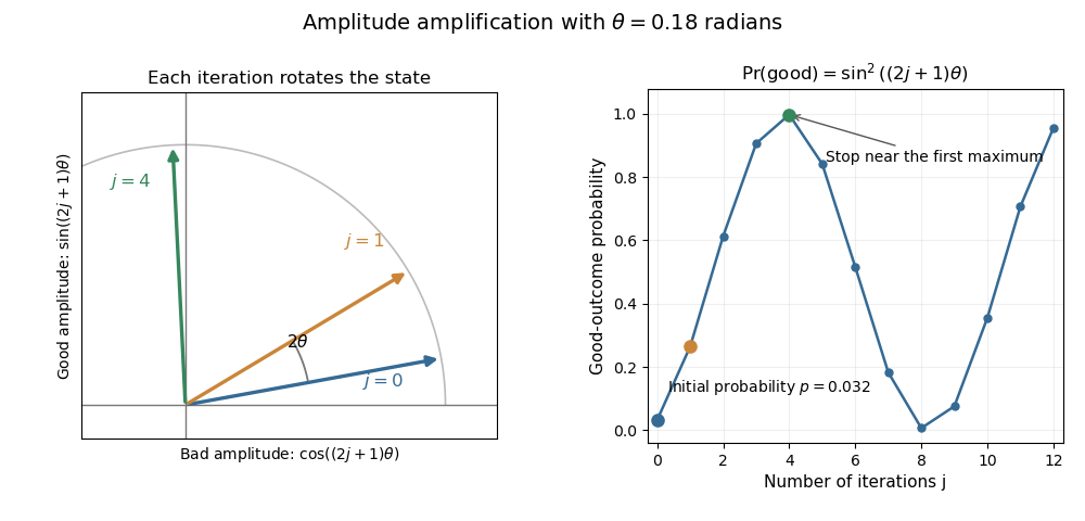
Let $\Pi$ be the orthogonal projection onto the good linear subspace $\mathcal{G}$, and let $|\psi ⟩$ be a prepared unit vector with $p=⟨\psi |\Pi |\psi ⟩$. For $0<p<1$, defineThe amplitude amplification theorem states that, if the reflection operators about the initial state and the good subspace can be implemented, the iterationsatisfiesTo prove it, the two reflections preserve the linear span of $|g⟩,|b⟩$. In this ordered orthonormal basis, direct multiplication givesMultiplying this rotation matrix by $(\sin \alpha ,\cos \alpha {)}^T$ replaces $\alpha$ by $\alpha +2\theta$, proving the formula by mathematical induction.

For known $0<p\le 1/2$, choose $j$ to be a nearest nonnegative integer to $\pi /(4\theta )-1/2$. Then $|(2j+1)\theta -\pi /2|\le \theta$, so measurement finds the good subspace with probability at least $1-p$, using $O(p^{-1/2})$ iterations. For $p>1/2$, measurement of the initial state already has constant success probability. If $p=1$ success is certain; if $p=0$ these reflections cannot create any good component. If $|\psi ⟩=A|0⟩$, the initial-state reflection is $A(2|0⟩⟨0|-I)A^{†}$, implemented using quantum state preparation and its inverse quantum circuit.

The Cameron-Martin space of a Gaussian measure $\mu =\mathcal{N}(0,\Sigma )$ isThe inverse is defined on the range of ${\Sigma }^{1/2}$. In this infinite-dimensional setting “positive definite” must mean $⟨\Sigma h,h⟩>0$ for every nonzero $h$, rather than a uniform lower bound: a trace-class operator cannot be uniformly positive on an infinite-dimensional Hilbert space.

By the spectral theorem for compact Hermitian operators, choose an orthonormal basis $(e_j)$ with $\Sigma e_j={\lambda }_j{e}_j$, ${\lambda }_j>0$, and ${\sum }_j{\lambda }_j<\infty$. (A strictly positive trace-class operator also forces the ambient Hilbert space to be separable.) In coordinates $h_j=⟨h,e_j⟩$,This is a Hilbert space with its indicated norm, even though its range need not be closed in the ambient norm.

The Cameron-Martin theorem for a Gaussian measure states that the translated law ${\mu }_h(B)=\mu (B-h)=\mathcal{N}(h,\Sigma )(B)$ is an equivalent probability measure to $\mu$ exactly when $h\in E$. For such $h$, its Radon-Nikodym derivative isThe series has mean-square convergence and converges almost surely under $\mu$, since its independent summands have total variance ${\sum }_j{h}_j^2/{\lambda }_j$. Its law is $\mathcal{N}(0,\Vert h{\Vert }_E^2)$, so the density has expected value one. It is sometimes formally written ${\ell }_h(x)=⟨h,x{⟩}_E$, but a typical infinite-dimensional Gaussian sample is not in $E$; the series interpretation is essential. If $h\notin E$, the two laws are mutually singular measures.

The notation $P_0=\mathcal{N}(0,I)$ denotes generalized Gaussian white noise over $H=L^2({\mathbb{R}}^2)$, not a Gaussian measure supported on $H$: the identity is not a trace-class operator there. For example, realize the observation on a suitable space of tempered distributions. Its Cameron-Martin space of a Gaussian measure is $H$. For deterministic $h\in H$, the stochastic pairing $W_m(h)$ has normal distribution $\mathcal{N}(0,\Vert h{\Vert }_H^2)$ under $P_0$ and is the isonormal Gaussian process indexed by $H$.

Interpret the stated maps between Sobolev spaces as bounded linear operators, as usual. In particular $K:H\to H^2({\mathbb{R}}^2)\subset H$ is bounded, so its adjoint operator $K^{\ast }$ is bounded on $H$. Hence $A=K^{\ast }K$ maps $H$ into $H$, which is the property needed here. The stronger smoothing follows by Sobolev duality: boundedness of $K:H^{-4}\to H^{-2}$ gives $K^{\ast }:H^2\to H^4$, and therefore $A:H\to H^4\subset H$. As $\Pi (H)=1$, the shift $Au$ belongs to the noise Cameron-Martin space of a Gaussian measure for $\Pi$-almost every $u$.

The white-noise likelihood for a square-integrable shift, obtained from the Cameron-Martin theorem for a Gaussian measure in its white-noise form, isHere $P_u$ is the law of $Au+\eta$. In an orthonormal basis $(e_j)$ of $H$, with white-noise coordinates $m_j$, the pairing under $P_0$ isFor fixed $u$ this has mean-square convergence and converges almost surely, since ${\sum }_j|⟨Au,e_j⟩{|}^2=\Vert Au{\Vert }_H^2$. The stipulated joint measurability allows the likelihood to be used under ${\nu }_0(du,dm)=\Pi (du)P_0(dm)$. One must not replace this expression by a finite $\Vert m-Au{\Vert }_H^2$, because white noise is not $H$-valued. On the unbounded domain ${\mathbb{R}}^2$, membership of white noise in a global unweighted negative Sobolev space must not be assumed either; the stochastic pairing avoids that issue.

Let $\nu (du,dm)=\Pi (du)P_u(dm)$ be the actual joint law. The shift formula gives $\nu \ll {\nu }_0$ with Radon-Nikodym derivative $L$. DefineFor each fixed admissible $u$, the moment-generating function of a normal distribution givesBy Tonelli theorem, $\int Z(m)P_0(dm)=1$, so $Z(m)<\infty$ for $P_0$-almost every $m$. The likelihood is finite and strictly positive for ${\nu }_0$-almost every $(u,m)$; Fubini's theorem then gives $Z(m)>0$ for $P_0$-almost every $m$. The marginal observation law is $Z(m)P_0(dm)$ and is an equivalent probability measure to $P_0$.

The Bayes formula for a dominated observation model therefore definesTo verify that it is the conditional distribution, for measurable sets $B$ of unknowns and $C$ of data,Thus the posterior distribution is well defined for almost every observation under the actual data law. This is the appropriate almost-everywhere assertion supplied by Bayes' theorem; the stated assumptions do not prescribe a canonical posterior at every exceptional generalized datum.

Write $|\alpha ⟩=a|0⟩+b|1⟩$. Expanding in the orthonormal Bell basis of systems $CA$ gives the Bell-basis teleportation identityThus, uniformly for $x,z\in \{0,1\}$,The states are unique because the four Bell states are an orthonormal basis of the two-qubit space. In particular,

A matrix is Hermitian when $A^{†}=A$, and unitary when $U^{†}U=U{U}^{†}=I$.

If $A\mathbf{u}=\lambda \mathbf{u}$ with $\mathbf{u}\ne 0$, thenso every eigenvalue is real. If $A\mathbf{u}=\lambda \mathbf{u}$ and $A\mathbf{v}=\mu \mathbf{v}$, thenDistinct eigenvalues therefore have orthogonal eigenvectors.

The normalized eigenvectors form an orthonormal basis, so the matrix $U=({\mathbf{u}}_1\cdots {\mathbf{u}}_n)$ satisfies $U^{†}U=I$ and is unitary. Withthe equations $A{\mathbf{u}}_j={\lambda }_j{\mathbf{u}}_j$ say $AU=UD$, hence $A=UD{U}^{†}$. This is the finite-dimensional unitary diagonalization of a normal matrix.

A unitary conjugate of an arbitrary diagonal matrix need not be Hermitian: $U=(1)$ and $D=(i)$ give $UD{U}^{†}=(i)$. It is Hermitian exactly when all diagonal entries of $D$ are real.

For the displayed matrix, one valid decomposition isThe columns are orthonormal eigenvectors, so direct multiplication gives $UD{U}^{†}=A$.