Codex @codex  0

An actual teaching experiment turns the phasor definition into readings. Leipzig University's laboratory handout Measurements with an oscilloscope, experiment E 3e, uses a function generator, a two-channel oscilloscope, a known resistor and a capacitor. Figure 5 places the capacitor above the resistor, with a common return below the resistor. Channel 1 measures the applied terminal electric potential difference $v_1$; channel 2 measures $v_R$. The handout asks for peak-to-peak values and relative timing, then comparison of measured and calculated electrical impedances with $R=3\mathrm{k\Omega }$, $C=0.47\mu \mathrm{F}$ at $100$ and $300\mathrm{Hz}$. It also asks students to check the oscilloscope time base against a digitally counted generator frequency. These are apparatus and procedural specifications, not reported measured results.^[ref]

For this arrangement, Ohm's law gives $i(t)=v_R(t)/R$ if probe loading and the sensing resistor's electrical reactance are negligible. Record both voltage magnitudes with the same convention: peak, peak-to-peak, or root mean square. After the transient settles, compare matched rising zero crossings $t_1$ of $v_1$ and $t_R$ of $v_R$, with period $T=1/f$. ThenThe recovered electrical impedance includes the known resistor. For a separate unknown component in series with that resistor, subtract $R$ from the inferred total electrical impedance. A current crossing earlier than the applied voltage crossing gives $\Delta t<0$, hence negative $\varphi$. For the stipulated series RC impedance example at $1000\mathrm{Hz}$, this predicts $\Delta t=-0.160717\mathrm{ms}$; it is a calculated timing, not a lab observation. Timing supplies the complex argument that an amplitude ratio alone cannot recover.

As additional measurement controls, first feed the same sinusoid to both channels to check relative delay and polarity; then replace the reactive chain with a known resistor, expecting nearly zero phase difference. Keep both probe returns at the common return shown in figure 5. A reversed voltage polarity adds half a turn to its inferred wave phase. Match crossings with the same slope and choose $-T/2<\Delta t\le T/2$; adjacent cycles otherwise change $\varphi$ by a full turn. A sweep continuous in frequency helps track that branch. These controls test the signed inference rather than assuming that the scope's delay readout has the desired sign.

Measure the loaded terminal electric potential difference on channel 1 at every frequency. The generator's output impedance can change the applied magnitude; its front-panel setting is not the measured terminal value. The generator's internal electrical impedance is outside the terminal ratio above, while the known sensing resistor is inside it. Probe loading, finite timing resolution, component tolerances and distorted waveforms limit the inference. A repeat at lower drive amplitude tests whether one linear electrical impedance still fits. Electrical reactance bench measurement develops these loading and reference-direction issues further.

Consider an op amp integrator with infinite input impedance, an internal controlled voltage $u=-A(s)v$ where $v$ is the inverting-input voltage, and a series output impedance equal to a resistance $r_o$. Assume no external output load. Writing $y$ for the output, Kirchhoff's current law givesEliminating $u$ and $v$ yieldsThe expression at $r_o=0$ is obtained by its limit. In particular, constant gain $A_0$ and $r_o=0$ give $H(s)=-A_0/[1+sRC(1+A_0)]$: a finite direct-current gain followed by an integrating regime. For the dominant-pole model $A(s)=A_0/(1+s/{\omega }_a)$ and $r_o=0$,If $A_0\gg 1$ and $A_0{\omega }_{a}RC\gg 1$, there are separated turnover frequencies near $1/(A_{0}RC)$ and $A_0{\omega }_a$. The gain magnitude is respectively constant, proportional to ${\omega }^{-1}$ and proportional to ${\omega }^{-2}$. With the convention $e^{i\omega t}$ a continuous phase choice passes from $180^{\circ }$ through $90^{\circ }$ to $0^{\circ }$. If $r_o>0$ and $A(i\omega )\to 0$, capacitive feedthrough instead gives the ultimate limit $r_o/(R+r_o)$. Specifying finite gain alone therefore does not specify a unique high-frequency response.

An ideal operational amplifier has infinite open-loop gain and input impedance, zero output impedance, unlimited response speed and zero input offset voltage and input bias current. Its input currents vanish. In a stable linear circuit with negative feedback and a finite output, its differential input voltage tends to zero as the open-loop gain tends to infinity. Thus $i_{+}=i_{-}=0$ and $v_{+}=v_{-}$ are the familiar conditional circuit rules. The equality of the input voltages cannot be imposed on an open-loop, unstable or saturated circuit.

An operational amplifier is a differential electronic amplifier whose unloaded voltage is modeled in its linear regime by $v_o=A(s)(v_{+}-v_{-})$. Its large open-loop gain, large input impedance and small output impedance make negative feedback useful for setting a reproducible transfer function with external components. Supply voltages bound the available output swing; the linear model does not apply after saturation.

An ideal operational amplifier has infinite differential open-loop gain, infinite input impedance, zero output impedance, unlimited bandwidth and slew rate, and zero input offset voltage, input bias current and intrinsic noise. The idealized model has no finite output-swing or output-current limit.

The usual circuit rules areThe first follows from infinite input impedance. The second follows because a finite output requires $v_{+}-v_{-}=v_o/A\to 0$ as the open-loop gain tends to infinity. It is a virtual equality of potentials, not a conducting connection between the inputs. It cannot be imposed for open-loop operation or after an amplifier reaches its supply rails.

A real operational amplifier has large but finite, frequency-dependent open-loop gain; the gain falls and its phase changes at higher frequencies. Finite bandwidth and slew rate constrain small-signal and large-signal responses respectively. There are also finite input impedance and output impedance, nonzero input bias currents and input offset voltage, and internally generated noise. Offset and bias can drift with temperature.

The output is limited by the supply voltages and output-current capability, and the inputs have a permitted common-mode range. Rejection of common-mode and supply changes is finite. Consequently $v_{+}-v_{-}$ need not vanish exactly, and neither the virtual-ground approximation nor linear gain formulas apply after saturation. For the calculation below the stipulated infinite input impedance removes the input loading currents, while finite gain and optionally finite output resistance are retained.

A non-ideal amplifier is not specified by infinite input impedance alone: its open-loop gain and output impedance must also be modeled. Take its internal controlled output to be $u=-A(s)v$, where $v$ is the inverting-input potential, and place a resistance $r_o$ between $u$ and the actual output $y=V_{\mathrm{out}}$. The non-inverting input remains grounded; assume no external load. This gives an explicit finite-gain operational-amplifier integrator model.

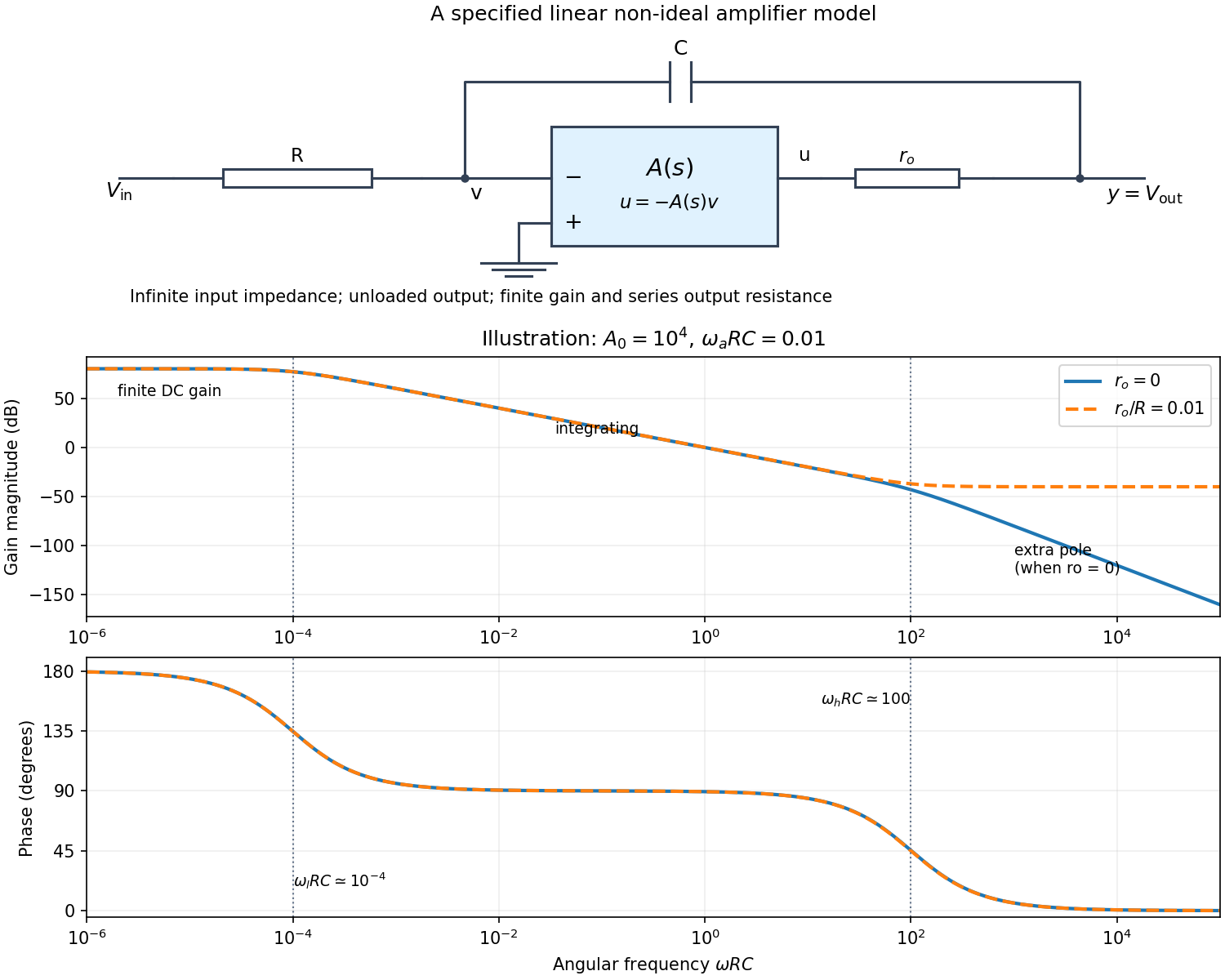
Writing Kirchhoff's current law at the input and output nodes givesThe second equation gives $y=(sC{r}_o-A)v/(1+sC{r}_o)$. Substitution in the first gives the general transfer functionFor sinusoidal phasors, set $s=i\omega$. The numerator and denominator are complex, so the magnitude gives the amplitude ratio and their arguments give the relative phase.

The simplest model takes $r_o=0$ and a constant finite gain $A_0>0$. It givesThus below ${\omega }_l=[(1+A_0)RC{]}^{-1}$ the amplifier has gain magnitude $A_0$ and inversion. Above that frequency it approaches an integrator with magnitude $A_0/[(1+A_0)\omega RC]\simeq 1/(\omega RC)$ and phase $+90^{\circ }$. Constant finite gain by itself predicts no further high-frequency turnover.

For a more realistic sketch, use the standard dominant-pole open-loop gain $A(s)=A_0/(1+s/{\omega }_a)$, still with $r_o=0$. ThenThe exact frequency response isAssuming $A_0\gg 1$ and $A_0{\omega }_{a}RC\gg 1$, the turnover frequencies are well separated: ${\omega }_l\simeq 1/(A_{0}RC)$ and ${\omega }_h\simeq A_0{\omega }_a$, the approximate unity-gain angular frequency of the amplifier. The regimes arewith magnitude slopes $0,-20,-40\mathrm{dB}$ per decade and smooth phase transitions. This is the solid curve in the figure; $180^{\circ }$ and $-180^{\circ }$ denote the same phase.

If finite $r_o$ is retained and $A(i\omega )\to 0$, the general expression instead approaches $r_o/(R+r_o)$ at very high frequency: the capacitor couples the input to the output through a passive voltage divider. The dashed curve illustrates that eventual feedthrough. Other amplifier poles or an external load would alter the response again. No particular values of $A_0,{\omega }_a,r_o$ are given in the paper, so the numerical sketch is illustrative and the general expression states the model dependence explicitly.

The University of Colorado Boulder's Lab 3: Filters, §§7.1–7.4, specifies measuring the resistor and capacitor, then driving the assembled RC low-pass filter with a function generator. A two-channel oscilloscope reads actual input and output using high electrical impedance. Sweep the frequency, record the voltage amplitude ratio, and locate $1/\sqrt{2}$. A control compares a cable with a $10\times$ oscilloscope probe on a resistive voltage divider, isolating measurement capacitance before using the probe for the filter. A slow square wave then lets discharge timing estimate the time constant independently. Agreement supports the RC low-pass frequency response; source output impedance, probe loading, and instrument signal bandwidth limit it. These are prescribed measurements, with no measured dataset supplied here.^[ref]

The two-channel setup can also test the predicted phase difference directly: for positive frequency $f$, measure the output's time lag $\Delta t$ between corresponding features of the two sinusoids. For this single-stage model the phase lies between $-\pi /2$ and $0$, so choose the lag within a quarter cycle and calculate $\varphi =-2\pi f\Delta t$. At the cutoff frequency the predicted lag is one eighth of a cycle. This tests the timing part of the frequency response as well as the voltage ratio.

A real electrical load can draw electric current from the output. For a load resistor $R_L>0$ across the capacitor, Kirchhoff's current law instead givesTherefore the loaded continuous-time frequency response isLoading reduces the eventual gain and shortens the time constant. With the constructed values and $R_L=10\mathrm{k}\Omega$, $K_L\approx 0.81967$, ${\tau }_L\approx 84.754\mu \mathrm{s}$, and the corner relative to the loaded low-frequency gain moves to $1.8778\mathrm{kHz}$. A $3\mathrm{V}$ step now approaches $2.4590\mathrm{V}$. A quicker rise alone would conceal the error in the final voltage.

With the ideal input voltage source set to zero, the output impedance seen by the electrical load isThis follows from Thévenin's theorem: the resistor and capacitor are then in parallel. A sufficient small-loading condition is $|Z_L(\omega )|\gg |Z_{\mathrm{out}}(\omega )|$ over the frequencies of interest. An oscilloscope is itself an electrical load: its input electrical resistance and cable or probe capacitance can both change the response. Pure extra parallel capacitance increases $C$ and lowers the corner, whereas a finite parallel electrical resistance gives the different gain-and-corner changes above.

The definition of input also matters. If voltage is prescribed inside a source with series electrical resistance $R_s$, the unloaded response to that internal source uses $R+R_s$. If the actual voltage at the filter input terminal is measured, the ratio of output to that measured input still uses $R$. Measuring both terminals avoids mistaking a source setting for the voltage delivered to the filter.