Past exam of the algebra, analysis and differential equations II course of the University of Oxford / 2004 (AC2, XMAT 4302, XMST 4302)

Source: Oxford mathematics examination release, ZIP member FOI-20210708-1 - Data/4302 (9).pdf. The printed cover identifies mathematics and mathematics and statistics. The complete editable transcription is retained in the private examination archive.

The dual basis is $E^{\ast }=\{e_1^{\ast },\dots ,e_n^{\ast }\}$, where $e_i^{\ast }(e_j)={\delta }_{ij}$ and each coordinate linear functional extends linearly. Thus $e_i^{\ast }({\sum }_j{a}_j{e}_j)=a_i$. These functionals are a basis of $V^{\ast }$ because a linear functional is uniquely determined by its values on $E$.

For a linear subspace $U$ of dimension $k$, extend a basis $u_1,\dots ,u_k$ to one of $V$. In its dual basis, the annihilator of a vector subspace $U^{\circ }$ is spanned by the last $n-k$ coordinate functionals. Hence $\boxed{\dim U+\dim U^{\circ }=\dim V}$.

The transpose in the source is the algebraic dual map $T^{\ast }:V^{\ast }\to V^{\ast }$ defined by $T^{\ast }f=f\circ T$. Composition of linear maps is linear, so $T^{\ast }f$ is a linear functional; and $T^{\ast }(af+bg)=a{T}^{\ast }f+b{T}^{\ast }g$, proving linearity in its input. If $T(e_j)={\sum }_i{a}_{ij}{e}_i$, thenThe coefficient of $e_j^{\ast }$ in $T^{\ast }{e}_i^{\ast }$ is consequently $a_{ij}$, so $\boxed{[T^{\ast }{]}_{E^{\ast }}=([T{]}_E{)}^{\mathsf{T}}}$. No inner product is involved.

A linear functional $f$ annihilates $\mathrm{Im}T$ exactly when $f(Tv)=0$ for all $v$, equivalently $T^{\ast }f=0$. Thus $(\mathrm{Im}T{)}^{\circ }=\ker T^{\ast }$. If $v\in \ker T$, then $(T^{\ast }f)(v)=f(Tv)=0$, giving $\mathrm{Im}{T}^{\ast }\subseteq (\ker T{)}^{\circ }$. The first equality and the dimension formula give $\dim \ker T^{\ast }=n-\dim \mathrm{Im}T$. By the rank-nullity theorem,The inclusion is therefore an equality:

The minimal polynomial of $T$ is the monic nonzero polynomial of smallest degree annihilating $T$. Such a polynomial exists, since sufficiently many powers of $T$ are linearly dependent in the finite-dimensional space $\mathrm{End}(V)$. If two monic annihilators had the same least degree, their difference would be an annihilator of smaller degree and hence zero. Thus it is unique. Division with remainder also shows that every annihilating polynomial is a multiple of it.

The primary decomposition theorem states that if $m={\prod }_{j=1}^r{f}_j^{e_j}$ with distinct monic irreducible polynomials, thenThese subspaces are $T$-invariant, and the restriction to $V_j$ has minimal polynomial $f_j^{e_j}$.

Let $r=\gcd (q,m)$, chosen monic. The Bézout's identity for polynomials gives $r=aq+bm$. If $q(T)v=0$, then $r(T)v=a(T)q(T)v+b(T)m(T)v=0$. Conversely, $q=rh$, so $r(T)v=0$ implies $q(T)v=0$. ThereforeThe following Roman scopes correspond to the three labelled conditions, with their implications proved from the indicated condition.

If a basis consists of eigenvectors, let ${\lambda }_1,\dots ,{\lambda }_r\in K$ be the distinct eigenvalues. A polynomial annihilates the diagonal action exactly when it vanishes at each ${\lambda }_j$. Consequently the minimal polynomial is ${\prod }_j(X-{\lambda }_j)$, a product of distinct linear factors. It therefore has no repeated irreducible factor, proving (i) implies (ii).

Suppose $m$ has no repeated irreducible factor. For every polynomial $p$ and integer $n\ge 1$, its monic greatest common divisors satisfy $\gcd (p^n,m)=\gcd (p,m)$, since raising $p$ to a power changes no membership of an irreducible factor of the square-free $m$. This is the square-free minimal polynomial criterion for polynomial kernel stabilization. The kernel identity proved above givesThus (ii) implies (iii) over every field.

Over $\mathbb{C}$, the distinct irreducible factors of $m$ are linear. The primary decomposition theorem therefore reads $V={⨁}_j\ker (T-{\lambda }_{j}I)$, a direct sum of eigenspaces. Taking a basis in each summand gives an eigenbasis, proving (ii) implies (i) over the complex numbers.

Over $\mathbb{R}$, take $T=\left(\begin{array}{cc}0& -1\\ 1& 0\end{array}\right)$. Its minimal polynomial is $X^2+1$, which is an irreducible polynomial over $\mathbb{R}$ and has no repeated factor. But it has no real eigenvalues, so no real eigenbasis. This is the required counterexample. Over a general field, the phrase “no repeated factors” here refers to irreducible factors in $K[X]$, rather than a prior assumption that those factors split.

Assume condition (iii), and factor $m={\prod }_j{f}_j^{e_j}$. If some $e_j\ge 2$, the primary decomposition theorem gives the nonzero summand $V_j=\ker f_j(T{)}^{e_j}$ on which the minimal polynomial is exactly $f_j^{e_j}$. The operator $f_j(T)$ cannot vanish on this whole summand, or its restriction would have minimal polynomial dividing $f_j$. Choose $v\in V_j$ with $f_j(T)v\ne 0$. Thencontradicting (iii) with $p=f_j$ and $n=e_j$. Hence every $e_j=1$, proving (iii) implies (ii).

An ideal is an additive subgroup $I\subseteq R$ with $rI\subseteq I$ for all $r\in R$. A ring homomorphism preserves addition and multiplication; for the rings with identity here use the standard unital convention $\theta (1_R)=1_S$. If $a,b\in \ker \theta$, then $\theta (a-b)=0$, and if $r\in R$ then $\theta (ra)=\theta (r)\theta (a)=0$. Thus the kernel is an ideal.

A maximal ideal is a proper ideal $I\ne R$ such that an ideal $J$ satisfying $I\subseteq J\subseteq R$ is either $I$ or $R$.

Use the standard definition that a prime ideal is proper, in addition to the product condition. The quotient operations areIts zero and identity are $I$ and $1+I$, which differ because $I$ is proper. If $(r+I)(s+I)=I$, then $rs\in I$, so primality gives $r\in I$ or $s\in I$. Thus one factor is zero. The commutative quotient ring has no nonzero zero divisors and is therefore an integral domain.

The printed definition omits properness. If that omission were read literally, $I=R$ would satisfy its product condition, but $R/I$ would be the zero ring, which is not an integral domain under the standard convention $1\ne 0$. Properness is the necessary qualification, retained explicitly in this proof.

The inverse image $I={\theta }^{-1}(J)$ is an ideal, by preservation of differences and multiplication. It is proper since $\theta (1)=1\notin J$. If $ab\in I$, then $\theta (a)\theta (b)\in J$; primality of $J$ gives $\theta (a)\in J$ or $\theta (b)\in J$, hence $a\in I$ or $b\in I$. Therefore the inverse image is prime.

For maximality, take the inclusion $\mathbb{Z}\hookrightarrow \mathbb{Q}$ and $J=(0)$. This is a maximal ideal of the field $\mathbb{Q}$, but its inverse image is $(0)$ in $\mathbb{Z}$, strictly contained in the proper ideal $2\mathbb{Z}$, so it is not maximal. Preservation of identity matters for proper inverse images: without it the zero homomorphism could pull a proper ideal back to the whole ring.

Use the boundary form of Cauchy's integral theorem: the integral of a holomorphic function around the oriented boundary of a compact region on whose neighborhood it is holomorphic is zero, including annular regions with the inner boundary oppositely oriented. Apply it to $f(z)/(z-a)$ between the circles of radii $r$ and $\rho$, both around $a$. It givesas $\rho \downarrow 0$, by continuity. This proves the Cauchy integral formula.

For a bounded entire function with $|f|\le M$, apply that formula at variable points inside a fixed circle and differentiate its kernel under the integral. At its center $a$, this givesThe circle can have any radius because the function is entire. Letting $R\to \infty$ gives $f^{\prime }(a)=0$ at every $a$, so $f$ is constant. This proves Liouville's theorem.

Finally, if a nonconstant entire function omitted all points within distance $ϵ$ of some $w$, then $g=1/(f-w)$ would be entire and bounded by $1/ϵ$. Liouville's theorem would make $g$, and hence $f$, constant. Therefore every such neighborhood contains a value of $f$, proving the dense image of a nonconstant entire function property.

Integrate $F(z)=e^{iz}/(z^2+1)$ around the real segment from $-R$ to $R$ and the counterclockwise upper semicircle, with $R>1$. The only enclosed pole is $i$, whose residue is $e^{-1}/(2i)$. On the semicircle, $|e^{iz}|\le 1$ and $|z^2+1|\ge R^2-1$, so its integral has magnitude at most $\pi R/(R^2-1)\to 0$.

The residue theorem thus gives ${\int }_{-\infty }^{\infty }{e}^{ix}/(x^2+1)dx=\pi e^{-1}$. The line integral converges absolutely, so taking its real part is justified:

For a nonnegative integer $n$, put $z=e^{i\theta }$ on the unit circle. Since $\cos \theta =(z+z^{-1})/2$ and $d\theta =dz/(iz)$,The residue at zero is the coefficient of $z^{2n}$ in $(1+z^2{)}^{2n}$, namely $\left(\genfrac{}{}{0ex}{}{2n}{n}\right)$. The residue theorem givesThe contour integrand has no other poles. The formula also includes $n=0$, giving $2\pi$.

A Möbius transformation is $M(z)=(az+b)/(cz+d)$ with $ad-bc\ne 0$, extended to the Riemann sphere at its pole and at infinity. Wherever its finite coordinate is defined,At a pole, the ordinary complex derivative is undefined, rather than zero; using the target coordinate $1/M$ gives a nonzero derivative there as well. Thus the source's nowhere-zero assertion is interpreted in local sphere coordinates, or on the finite domain with the pole excluded.

Composition corresponds to multiplication of the invertible matrices $\left(\begin{array}{cc}a& b\\ c& d\end{array}\right)$, with scalar multiples giving the same map. The identity matrix gives the identity, and the inverse matrix gives an inverse Möbius map. This proves the group property on the Riemann sphere.

The two boundary circles meet at $\pm i$. PutFor $w=u+iv$, direct substitution givesThis gives a lens-to-half-plane map through the intersection points. Both lens inequalities hold exactly when $u<-|v|$, the open sector with continuous argument between $3\pi /4$ and $5\pi /4$. This proves bijectivity, since the inverse is defined throughout that sector and the excluded endpoint $-i$ is not in the lens.

Rotate the sector through $-3\pi /4$ and square it, obtaining a bijection onto the upper half-plane. Therefore a conformal map isSquaring is injective on this sector because it contains no pair of opposite points. Its derivative and the Möbius derivative are nonzero in the interior, so the bijection is conformal.

A critical point of a dynamical system is a point where both components of the vector field vanish. For a continuously differentiable vector field, strictly negative real parts of both eigenvalues of its Jacobian matrix imply asymptotic stability of the equilibrium. If an isolated critical point is a center of a planar dynamical system and the eigenvalues are distinct, they must be a nonzero purely imaginary conjugate pair. Purely imaginary eigenvalues alone do not in general prove nonlinear stability; the nonlinear ordinary differential equation system must still be examined.

Here the critical points are $(0,0)$ and $(\pm 1,0)$, with Jacobian $\left(\begin{array}{cc}0& 1\\ 1-3x^2& 0\end{array}\right)$. At zero its eigenvalues are $1,-1$, giving an unstable saddle equilibrium. The unstable direction is $(1,1)$ and the stable direction is $(1,-1)$. Thus trajectories leaving the origin are tangent to $y=x$, and those returning are tangent to $y=-x$, with both opposite rays included.

An exact first integral isThe two homoclinic loops belong to $H=0$:They confirm the incoming and outgoing tangent directions. For example the right loop is $x=\sqrt{2}\mathrm{sech}(t-t_0)$, $y=-\sqrt{2}\mathrm{sech}(t-t_0)\tanh (t-t_0)$; changing both signs gives the left loop.

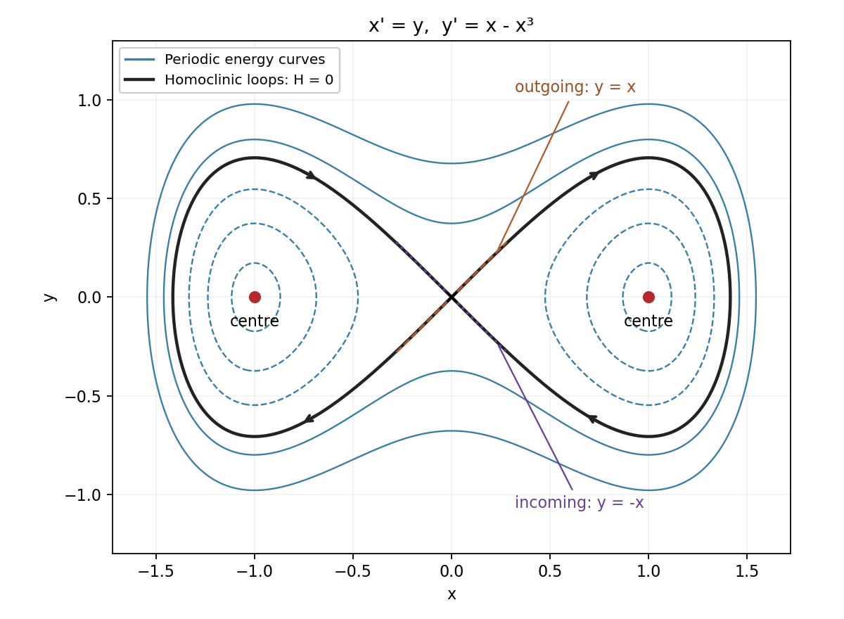
At $(1,0)$ put $x=1+X$, $y=Y$. The exact equations are $X^{\prime }=Y$, $Y^{\prime }=-2X-3X^2-X^3$, so the linearization of a dynamical system gives $X^{\prime \prime }+2X=0$. Its nonconstant solutions haveThe same linear classification holds at $(-1,0)$. For the nonlinear ordinary differential equation system, $H$ has strict local minima $-1/4$ at both points. Levels $-1/4<H<0$ are two families of smooth closed ovals, proving that both are stable centers, rather than asymptotically stable equilibria. These give actual periodic orbits of the nonlinear ordinary differential equation system, with small-amplitude periods tending to $\sqrt{2}\pi$.

The method of characteristics usesFor a graph parametrized by $(x,y,u(x,y))$, a normal vector is $N=(-u_x,-u_y,1)$. The PDE says $N\cdot (a,b,c)=0$, so the characteristic vector is tangent to the solution surface. Flowing a suitable initial curve along these directions constructs a surface; where its projection to the $(x,y)$ plane has nonzero Jacobian determinant, the inverse function theorem makes it a graph. Local uniqueness of this general flow needs the usual regularity assumptions beyond mere continuity. The particular characteristic system below is smooth and can be solved explicitly.

Label the initial points by $\eta \ge 0$. Since $dx/ds=1$, take $x=s$. The other two equations integrate toEliminating $\eta =y-xu+x^3/3$ gives the implicit solutionFor each fixed $|x|<1$, the derivative of the displayed $y$ with respect to $\eta$ is $1+x\cos \eta \ge 1-|x|>0$. It increases from its value at $\eta =0$ to infinity, so it is a bijection from $[0,\infty )$ onto $[y_L(x),\infty )$, whereThus there is exactly one characteristic label, and hence one solution value, throughout the requested region, including the initial-label boundary as a trace.

The characteristic fold for sinusoidal data in a forced Burgers equation is seen by differentiating with respect to $y$:For a fixed integer $k\ge 0$, let $y_{\ast }=(2k+1)\pi +7/6$. As $x\to 1^{-}$ at this fixed $y_{\ast }$, the label tends to $(2k+1)\pi$, giving $u_y\to -\infty$. To justify the label limit, the limiting map at $x=1$ is strictly increasing despite isolated zero derivatives, so its inverse has a unique continuous limit. Similarly, at any fixed $y_{\ast }=2k\pi -7/6$ with $k\ge 1$, the limit as $x\to -1^{+}$ has $\eta \to 2k\pi$ and $u_y\to +\infty$. These fixed values lie within the region near the respective boundary, proving the requested gradient blow-up.

The derivative formula requires additional regularity: continuity alone does not define $f^{\prime }$. Assume $f$ is continuously differentiable, or locally absolutely continuous with its almost-everywhere derivative. Integration by parts on $[0,R]$ givesFor $\mathrm{Re}p>c$, the given exponential bound makes the first term tend to zero. Thus the improper transform exists under these regularity assumptions andFor the primitive, absolute integrability justifies reversing the integration order:Indeed the corresponding absolute double integral is finite when $\mathrm{Re}p>c$.

For real $p>0$, substitution $t=s^2/p$ and the supplied Gaussian integral giveBoth sides are holomorphic for $\mathrm{Re}p>0$, so the identity theorem extends this equality there, taking the square root with positive real part. The integrable singularity at zero causes no difficulty for this improper integral. The primitive rule then gives $\mathcal{L}[2\sqrt{t}]=\sqrt{\pi }{p}^{-3/2}$.

For the conductor, take the Laplace transform in time and write $U(x,p)$. The initial temperature gives $U_{xx}=pU$. Use the usual physical condition that the temperature is bounded far down the conductor; this selects the decaying solutionThe constant applied flux has transform $Q/p$, so $-k{U}_x(0,p)=Q/p$, giving $A(p)=Q/(k{p}^{3/2})$. This is the surface temperature under constant heat flux on a half-line. Using the transform just calculated yieldsHere $k>0$ is the thermal conductivity. The far-field boundedness is the customary physical selection condition; without a spatial growth restriction the written PDE and initial/boundary data alone do not specify that selection. Within the physical solution, the face temperature tends continuously to zero as $t\downarrow 0$.