Let be the energy of one adsorbed atom, using the same energy reference as the gas-phase value . For equivalent, noninteracting adsorption sites, choosing the occupied positions givesEvery configuration has energy , so the canonical lattice-gas partition function isThere is no further factor: the combinatorial choice already counts indistinguishable adsorbates correctly. The Helmholtz free energy, using Stirling's approximation for a macroscopic number of occupied and empty sites, isHence the adsorbed-phase chemical potential at fixed isThe logarithm comes from configurational entropy: adding an atom is less favorable when vacancies are scarce. In the gas, the stipulated expression can be writtenwhere is the thermal de Broglie wavelength. Equality of chemical potentials at chemical equilibrium givesThereforeThe binding energy is positive for favorable binding. The units of are inverse pressure, making dimensionless. Choosing the adsorbed energy as zero simply sets and leaves the same physics; it must not remove the relative binding energy. This is the Langmuir isotherm, with low-pressure linear uptake and high-pressure monolayer saturation.
At chemical equilibrium, adsorption and desorption balance:Canceling and rearranging givesThus when the kinetic and thermodynamic descriptions refer to the same ideal surface and energy convention. In particular,The ratio fixes the adsorption isotherm, while the individual rate constants also determine relaxation toward equilibrium. Here has units of inverse pressure per time and of inverse time, so is dimensional. This equivalent-site arrival/departure argument is the simple case of the Langmuir adsorption model.[ref]
The Adsorption of Gases on Plane Surfaces of Glass, Mica and Platinum by Irving Langmuir. theoretical part, Case I, pp. 1368–1370: equivalent elementary surface spaces and equilibrium adsorption
For the uniform-binding multilayer adsorption model, describes sites of exactly height , not the fraction whose height is at least . At equilibrium the upward and downward fluxes on each adjacent pair of heights balance:For completeness, stationarity alone gives a height-independent probability current; the reflecting boundary at height zero sets that current to zero. This justifies pairwise balance for a normalizable equilibrium distribution.
Writing gives the recurrence . Successive substitution then yieldsAn equilibrium geometric distribution of unbounded heights requires . The first-layer-only Langmuir adsorption model instead truncates the allowed heights at one, which changes the normalization and removes this convergence restriction.
Normalizing the geometric distribution requiresThere are sites containing atoms each. Therefore the expected total population isConsequentlyThe quantity counted is the total number of atoms in every layer. The number of nonempty columns is instead .
Dividing the total adsorbed population by the number of underlying adsorption sites givesThis multilayer uptake can exceed one because it is a mean column height. The occupied-site fraction remains . If each layer has the same binding energy and microscopic states assumed in the single-layer calculation, the corresponding thermodynamic expression for is also the one obtained there; the kinetic ratio is the definition supplied by this multilayer model.
The model allows unlimited column height without weakening the binding or reducing the upward rate as a column grows. As , successive heights become nearly equally probable and the mean height diverges. At , the putative height weights cannot even be normalized; for they increase with height and no finite stationary uptake exists.
This is a condensation-like failure of the unbounded-layer idealization, rather than a monolayer reaching its capacity. Finite gas supply, finite geometrical capacity, altered layer binding and interactions can modify or limit the actual uptake. The divergent expression is an equilibrium result only below its convergence threshold.
Choose the ground-state energy as zero and write . The molecular partition function must sum individual states, so the triply degenerate excited level contributes three Boltzmann factors:The probabilities of occupying the two levels areEach of the three individual excited states has probability . At high temperature the four states become equiprobable, so the two levels have probabilities and , not each. This is the distinction between a level and its state degeneracy.
Use the additive-volume two-level system implicit in the model: each excited particle increases the volume by the same increment. The difference between the two endpoint volumes is , so that increment is .
If particles are excited, . Linearity of the expectation gives , henceAs , . As , only three quarters of the particles are excited on average, giving , rather than the all-excited endpoint . These limits also check the inclusion of state degeneracy.
The definition uses a fixed reference volume, so it is a reference-volume thermal expansion coefficient:Let . Sincewe obtainIt is positive and has units of inverse temperature. Equivalently, : the response reflects changes in the thermally occupied excited population. The usual instantaneous fractional thermal expansion coefficient would instead equal ; substituting that different definition would change the answer.
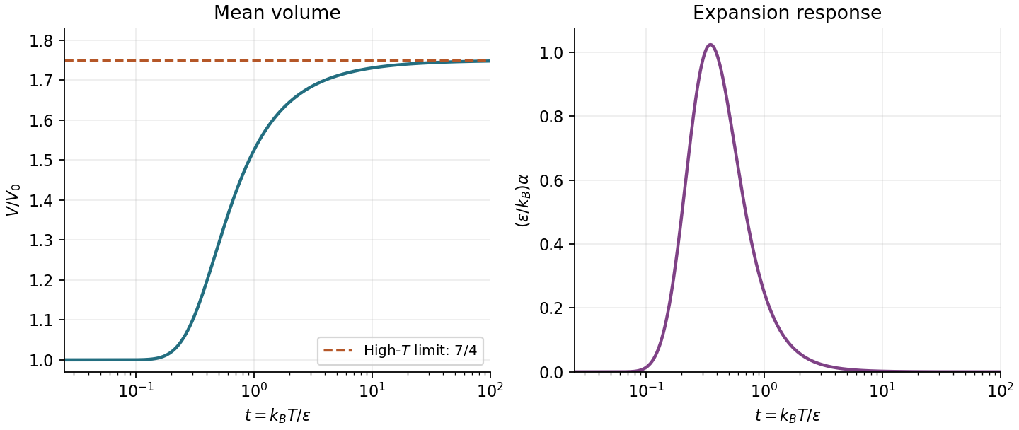

At low temperature, , so the denominator in the exact expression approaches one:The exponential suppression dominates the factor. Almost all particles remain in the ground state, so very little volume change is thermally accessible.
At high temperature, , and thereforeThe excited fraction has already approached , so further heating barely changes it. Both limits are consistent with a bounded two-level system; the high-temperature vanishing does not imply that ordinary materials cease expanding when additional levels or other mechanisms become accessible.
For an ideal mixture, the Helmholtz free energy is a sum over species. At fixed and all other populations, the molecular partition function does not depend on . Differentiating the contribution written using each species' own energy reference givesThe desired additive energy term requires a consistent energy reference in molecular partition functions. Let be the energy per molecule of species in its reference state, measured relative to a common chemical energy zero, and let sum excitations above that reference. ThenThereforeOne convenient choice is each species' rovibrational ground state, so the molecular reference includes its zero-point energy. A different consistent reference is possible, but the corresponding partition function must change. The offset cannot arise from differentiation of a formula that has already omitted it, and it must not be counted twice. These chemical potentials are per particle; molar expressions instead use the molar gas constant.
For an ideal gas, translation makes the molecular partition function proportional to volume. Define the molecular partition function density and number concentration byThenBoth and have units of inverse volume, so their ratio is dimensionless. If concentrations are specified in moles per volume instead, replace in this microscopic expression by times that molar concentration, with consistent volume units.
At chemical equilibrium, . Using the number-concentration form givesHere is the reaction energy between the chosen molecular reference states. Rearranging,Define the dimensionless concentration equilibrium constant byThusThe standard concentration has the same units as . It converts concentration ratios to ideal thermodynamic activities; changing it changes the numerical dimensionless for this dissociation, which creates an extra particle. The unnormalized quotient instead has concentration units.[ref]
IUPAC Compendium of Chemical Terminology (Gold Book) by International Union of Pure and Applied Chemistry. entries equilibrium constant and standard equilibrium constant: distinguish concentration quotients from the thermodynamic dimensionless standard constant
First construct the energy cost for heterolysis from the molecular potential minimum. Dissociation to neutral atoms costs , ionizing caesium costs , and attachment of the electron to iodine releases EA. ThereforeFor the ground-state reference convention used above, the initial molecule already has vibrational zero-point energy. Thus its ground-state dissociation energy is andAt , , givingAlternatively, retaining the molecular minimum as reference gives and a Boltzmann factor . That convention must use the full vibrational partition function, including , in the next part. The ground-state convention instead uses . Either consistent convention gives the same final equilibrium constant; using the ground-state reaction energy with the full zero-point factor would count the correction twice. The distinction between and is a distinction between initial states, not a change in the dissociation products.[ref]
IUPAC Compendium of Chemical Terminology (Gold Book) by International Union of Pure and Applied Chemistry. dissociation energy and bond-dissociation energy in theoretical chemistry: well-minimum and ground-state energy conventions
Use ground-state references and the supplied ideal-gas, rigid-rotor and harmonic-oscillator approximations. The two ions have closed electronic shells; take their electronic ground-state degeneracies and the molecular electronic ground-state degeneracy as one, and neglect higher electronic levels. Consistently treated nuclear-spin factors cancel between the species. Since the molecule is heteronuclear, its rotational symmetry number is one.
Let be the reduced mass, neglecting the negligible mass correction from electron transfer. The ratio of translational partition functions per volume reduces toThe molecule has additional rotational and vibrational states, whereas the monatomic ions do not. At ,Hence the dimensional equilibrium quotient isThe last form makes the unassigned standard concentration explicit. For the common choice of , the corresponding microscopic reference is , givingEquivalently, the dimensional molar quotient is . A pressure-based gas standard is a different convention: taking with would give , rather than the same numerical constant.
The well-minimum convention gives the identical answer becauseConstants used here are , , and .[ref]
CODATA recommended values of the fundamental physical constants: 2022 by National Institute of Standards and Technology. fundamental-constant tables: Planck constant, Boltzmann constant, atomic mass constant and Avogadro constant
The stipulated conventional cell is a square of side . Although introduced as a centered rectangular lattice, this equal-side case is a square Bravais lattice viewed with a rotated primitive basis. A corner-to-center separation iswhich is shorter than the separation between adjacent conventional corners. Consequently the first contact of equal circles occurs atThe conventional square represents two lattice points: one from its four shared corners and one from its center. Its packing fraction is thereforeEquivalently, one circle occupies each primitive area . This is square circle packing; the drawing does not define a triangular close-packed lattice.
A unit cell is a repeat region whose lattice translations tile the plane. A primitive unit cell represents exactly one lattice point and has the minimum repeat area for a lattice basis.
Cell A is nonprimitive; cell B is primitive. A represents two points and has area . B has four shared corner points and no additional interior point, represents one point and has area . Fractional corner counting refers to the tiling, not to fractional physical atoms.
Using the printed axes, take a lower vertex of cell B as origin. One allowed pair of primitive lattice translation vectors isBoth vectors connect nearest lattice points, have length , and are perpendicular. Their determinant has magnitude , consistent with a primitive area. Exchanging them or reversing their directions gives equivalent basis conventions; the corresponding reciprocal lattice vectors must then use the same convention.
A visibly different primitive parallelogram is generated byIts vertices, relative to one lattice point, are , , and . Its area isThe basis change has integer matrix with determinant one. It is invertible over the integers, so the new vectors generate every original lattice point, not merely a sublattice. The cell is therefore primitive despite being sheared relative to cell B.
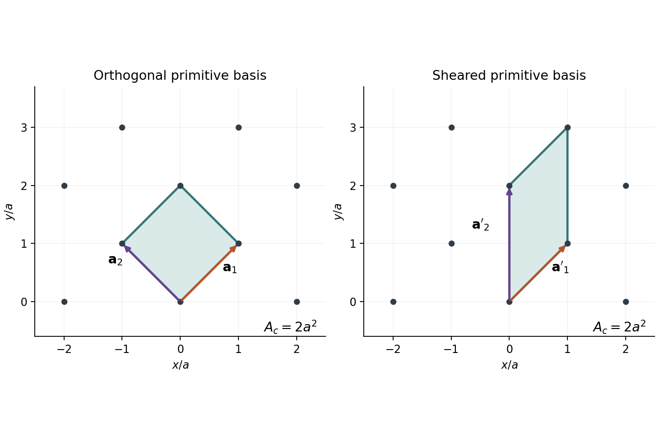
Two primitive bases generate the same centered-square lattice
. Original coordinate construction from the derived translation vectors, with axes measured in units of . The left cell uses the diagonal orthogonal basis; the right uses a determinant-one shear. Both highlighted parallelograms have area and one lattice point per cell. Details.
For direct-lattice points , a lattice-periodic plane wave must have the same phase at every translated lattice point:Thus , with integer , and the reciprocal lattice isIts spacing is . These plane waves execute an integer number of complete cycles within a direct-lattice period, so their wavelength magnitudes are for .
A general electronic Bloch wave need not itself be lattice-periodic: wavevectors differing by have the same translation phase. The reciprocal lattice labels that equivalence, while a large finite specimen with periodic boundary conditions has a much finer grid of allowed electronic wavevectors.
Construct Bragg planes by taking the midpoints between the reciprocal origin and the other reciprocal lattice points. In one dimension these are points at , for nonzero integer .
The first Brillouin zone is the interval bounded by the nearest two such points:The second Brillouin zone consists of the next intervals on both sides:Boundary points may be assigned to one adjacent zone to avoid double counting. The first zone is reached from the origin without crossing a Bragg point; the second is reached after crossing one. Each zone has total length . In particular, the two separated pieces of the second zone are not the entire translated first-zone interval centered at .
With the chosen basis, let . The reciprocal lattice conditions giveso . Similarly, and giveAll reciprocal points areThus, in coordinates measured in , the two integer coordinates have the same parity. The reciprocal lattice is another rotated square Bravais lattice, with nearest-neighbor spacing .
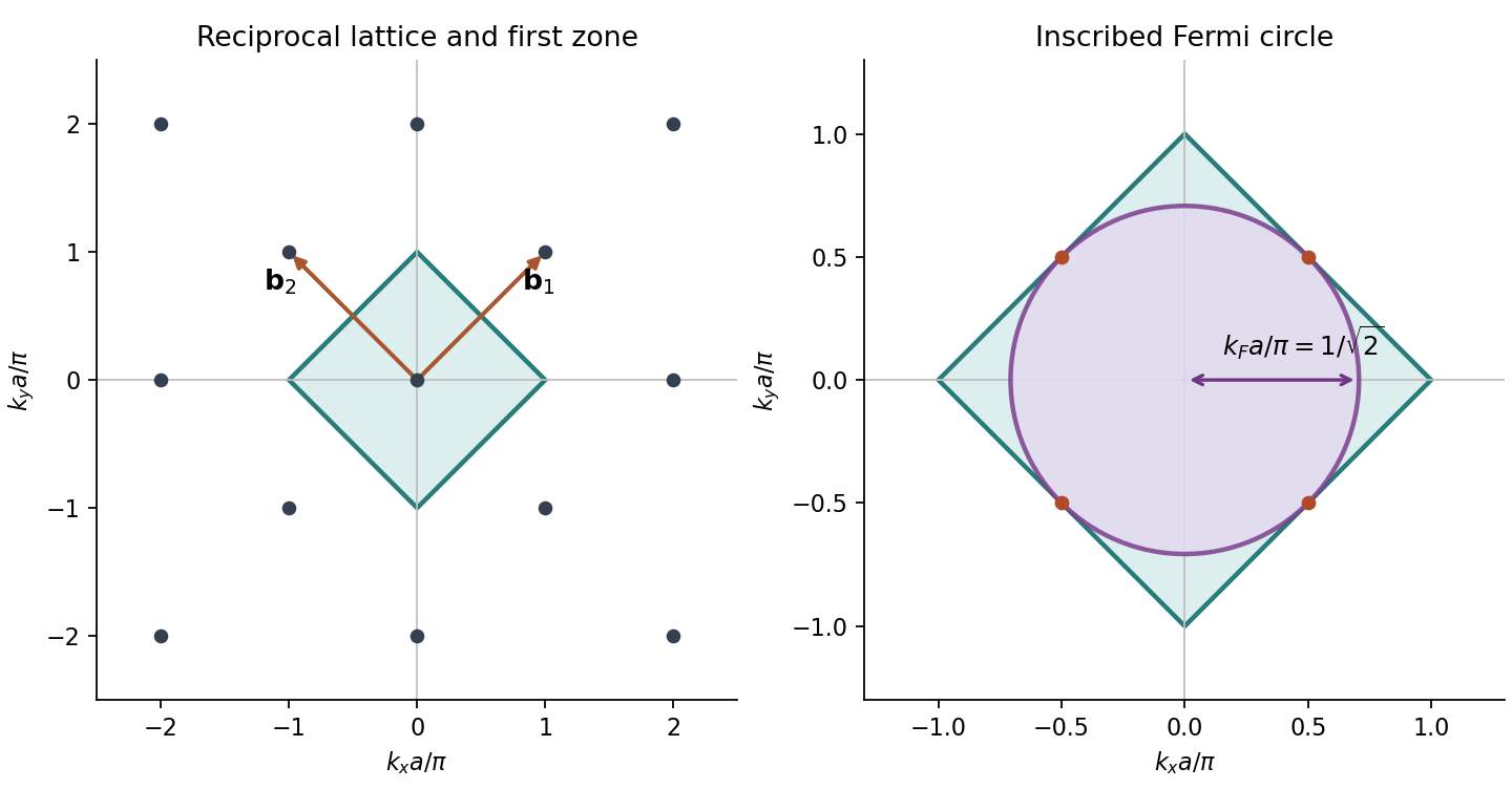

The first Brillouin zone is the origin-centered Wigner-Seitz cell of the reciprocal lattice. Its nearest reciprocal points are and . The perpendicular bisectors follow fromConsequently the zone isIt is the diamond with verticesThe reciprocal-space sketch above shows these boundaries. Its area is , where . This area check rules out mistakenly using the nonprimitive conventional cell to define a smaller first zone.
For an isotropic two-dimensional free-electron model, the occupied states form a disk centered at the reciprocal origin. Its Fermi circle first touches a zone side when its radius equals half the distance to a nearest reciprocal point:The contact points have coordinates with all four sign combinations. The distance to a zone vertex is , which is larger; that distance would describe contact with a corner after the circle had already crossed a side.
There are primitive cells and therefore lattice points. The specified reciprocal-space density counts distinct allowed wavevectors; each supports two electron spin states. Filling the disk at zero temperature givesUsing and ,The circle fills a fraction of the first-zone area, while one spin-degenerate band has two states per primitive cell; these give the same result. A single-spin count would instead be , omitting the physical twofold spin degeneracy of this model. The circle has only just reached the sides, so the zone corners remain unfilled: first contact does not mean filling the entire first band.
The density of states counts available one-electron states: is the number with energies in . It describes the spectrum, irrespective of whether those states contain electrons.
The density of occupied states additionally weights each state by the Fermi-Dirac distribution:Thus is the mean number of electrons in that energy interval, and . State and electron densities must use the same normalization, including whether they are extensive or per volume and whether already includes spin degeneracy. The symbol here denotes occupied density, not a canonical partition function.
The finite-temperature Fermi level lies at the middle of the gap in the stipulated symmetric intrinsic model:Here is the valence-band maximum and the conduction-band minimum. Thermal promotion creates one conduction electron and one electron hole, so charge neutrality requires . Equal constant densities of states in broad, symmetric bands give equal populations when the distances and are equal.
This is a statement about the chemical potential, not an available electron state in the gap. Unequal band densities of states would shift the intrinsic Fermi level away from exact midgap; the equality follows from the symmetry assumed here.
Heating promotes electrons across the band gap, creating mobile conduction electrons and electron holes. Their contributions add:where are the electron mobility and hole mobility, and is the positive elementary-charge magnitude. The increase in carrier density gives the rising electrical conductivity in the intrinsic activation regime. Mobility need not itself increase with temperature; the model attributes the dominant increase to carrier generation.
Let be the equal constant density of states per unit volume and energy in each band. In the nondegenerate semiconductor regime, the conduction-band occupation isFor bands broad compared with , integrating above the conduction edge givesThe valence-hole integral similarly gives . Midgap therefore impliesInserting the carrier densities into the transport expression yieldsOn treating the algebraic and mobility prefactor as approximately constant, the requested leading activation law isThe factor is essential: an intrinsic excitation creates an electron–hole pair, and charge neutrality places the chemical potential halfway across the symmetric gap. The conduction-electron population is governed by , not by replacing this separation with the full gap.
There is a qualification to the proportionality as printed. A literal constant-density-of-states intrinsic semiconductor with temperature-independent mobilities retains the additional factor . Indeed, using the full Fermi-Dirac distribution giveswhich reduces to the expression above when . Thus the pure exponential is an activation approximation, not an exact consequence of constant DOS alone. A mobility sum proportional to would cancel the leading algebraic factor.
Using the requested exponential law with a temperature-independent prefactor,The conductivity ratio is two, soThe denominator is positive, as required for a positive gap and rising conductivity. If one instead retains the constant-DOS factor while keeping mobility constant, the inferred gap becomesThat is a different prefactor model; is the estimate from the relation specified for this part.
Arsenic has five valence electrons, whereas silicon has four. A substitutional arsenic atom can therefore supply an extra electron after participating in the silicon bonding network. It acts as a shallow donor impurity, introducing a localized level just below the conduction band. Ionizing that donor costs much less energy than excitation across the full band gap.
At the lowest temperatures, donor electrons remain bound and the valence band is filled. Mobile-carrier populations are negligible: this is dopant freeze-out. Initial heating releases donor electrons into the conduction band, producing a rapid rise in conductivity governed by the shallow-donor energy scale. The positive ionized donor charge compensates the released electronic charge; the bulk need not acquire net charge.
At intermediate temperatures, nearly all donors are ionized but intrinsic electron–hole generation is still small. In an uncompensated sample,where is donor number density. The supply of donor electrons is finite, so further heating cannot keep creating them. This is the extrinsic plateau under the approximation of weakly varying mobility, and its carrier density is much larger than that of the undoped sample at the same temperature. In real material, scattering changes mobility, so donor exhaustion alone predicts a carrier-density plateau rather than guaranteeing perfectly flat conductivity.
At higher temperatures, intrinsic generation becomes comparable to and then exceeds the donor contribution. Once , the populations approach , and activation across the main gap causes the steeper rise. The relevant regimes are therefore freeze-out, donor exhaustion, and intrinsic excitation, not three successive types of dopant.
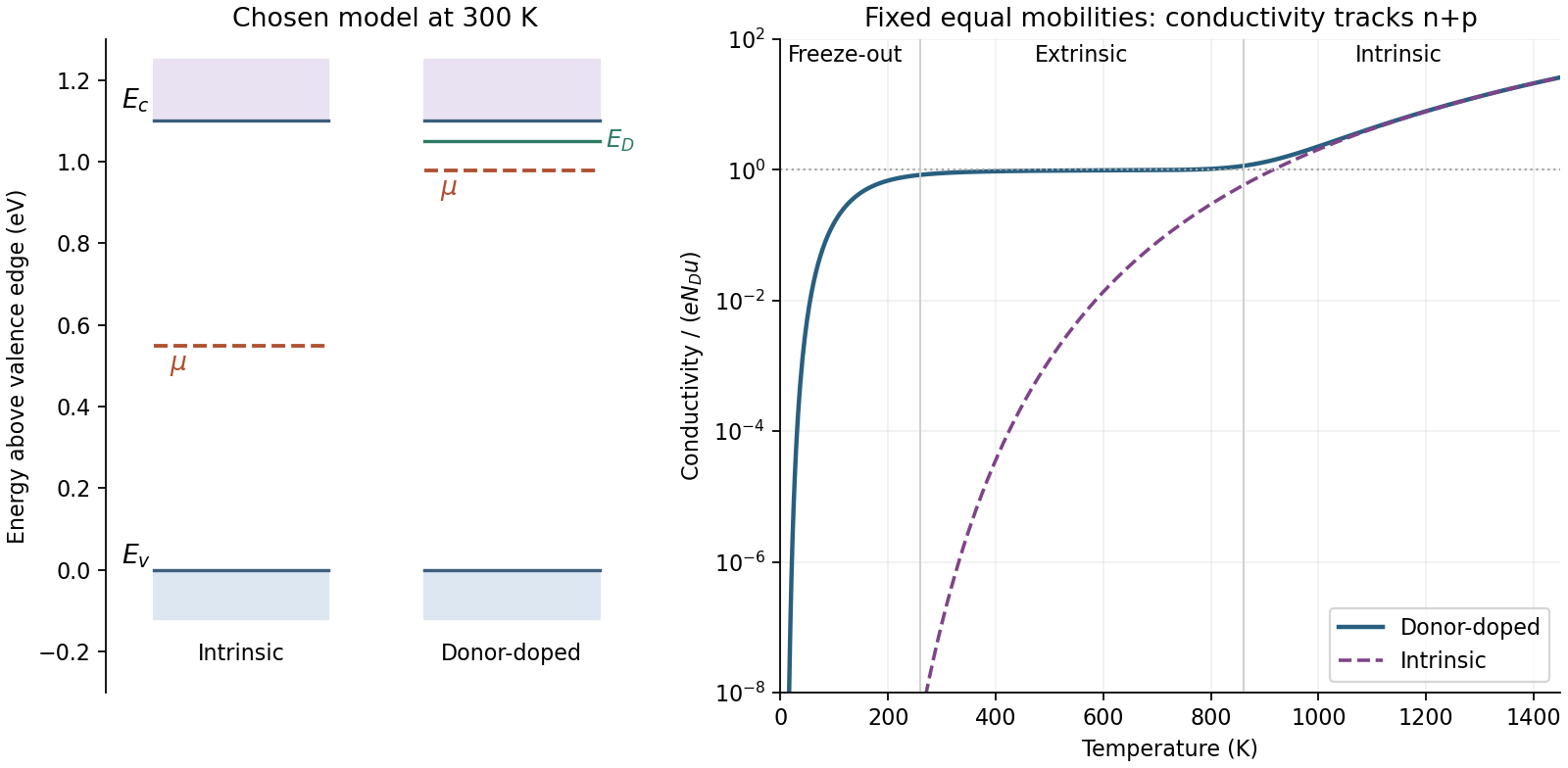
Donor occupation, Fermi-level position and three conductivity regimes
. Original illustrative model, not measurements of arsenic-doped silicon. The right panel solves charge neutrality with partial donor ionization and intrinsic carriers, assuming fixed equal electron and hole mobilities. Chosen parameters are , donor binding and . The left panel illustrates the resulting room-temperature energy ordering, including a Fermi level below the donor level. Details.
The ambient-temperature Fermi level is raised into the upper part of the gap, toward the conduction-band edge, relative to intrinsic silicon. The sample is an n-type semiconductor: ionized donors supply many more conduction electrons than the intrinsic population.
For a nondegenerate, substantially ionized sample with negligible acceptors, . With effective density of states , the conduction-band relation givesBecause a few ppm normally gives at ambient temperature, the chemical potential remains below the conduction-band edge rather than entering it as in a strongly degenerate semiconductor. Its precise position requires the dopant density, density of states and degree of ionization; the broad qualitative shift is fixed by donor doping.
It is not necessary for to lie between the donor level and the conduction edge. In a substantially ionized nondegenerate sample, the chemical potential can lie below the shallow donor level, as in the illustrative diagram. Donor ionization is determined by the level's occupation relative to ; a finite-temperature Fermi level is not the highest filled one-electron level of every individual configuration.
Articles by others on the same topic
There are currently no matching articles.