Source paper: Oxford public bundle, pages 72–74. The bundle filename says 2016, but the held B6 cover is dated 10 June 2017. All four options are solved. Letters below identify successive unlettered source paragraphs; the inline Roman labels are retained.
With the convention , the reciprocal lattice of a face-centered cubic lattice is a body-centered cubic lattice. The reciprocal conventional cube is parallel to the direct conventional cube and has side . In direct-cubic coordinates its points areThe even triples supply the corners of that reciprocal cube and the odd triples its body centres. The atomic basis can change diffraction intensities through its structure factor; it does not change the reciprocal lattice determined by the translation lattice.
The cubic Miller indices give an interplanar spacing . Equivalently, the reciprocal lattice vector normal to these lattice planes has length . HenceThe eight reciprocal lattice vectors are the nearest nonzero reciprocal points. Their perpendicular bisectors form the eight hexagonal faces of the first Brillouin zone, a truncated octahedron. For the positive direction, that Bragg plane is , or . It is parallel to the direct lattice planes. The six remaining square zone faces correspond to the reciprocal points. The zone boundary is halfway to a reciprocal point, not the point itself.
Use the angle between two planes defined as the acute angle between their normal vectors. The normals and have dot product one and lengths . ThusChoosing an oriented rather than an acute interplanar angle could give the supplementary ; it describes the same unoriented pair of lattice planes.
The normal vector is . Its normalized dot product with is , soThis is the acute angle between the lattice planes, rather than the complementary angle between a plane and the other plane's normal.
The X-ray wavelength is . Write the amplitude of one conventional unit cell as the face-centred cubic selection rule times the two-atom atomic basis amplitude:The first bracket is four when the indices have equal parity and zero otherwise. Among the allowed Bragg reflections, the zinc blende structure factor therefore givesHere the atomic scattering factors are taken as real. For the requested rough estimate set and . The weak difference reflections remain allowed: unequal species do not have the extra exact extinction of the equal-species diamond limit.
The first six allowed values of are . Bragg's law gives the measured scattering angle . For powder diffraction, multiply the squared amplitude by the powder diffraction multiplicity . The last two columns use :The first intensity column is the geometry-independent multiplicity-and-structure estimate. The second additionally assumes an unpolarized beam and a common symmetric powder-diffractometer geometry, with Lorentz-polarization factorAn overall constant cancels in either normalization. A particular measured intensity set is not fixed by the atomic numbers alone: actual atomic scattering factors decrease with momentum transfer, anomalous scattering and absorption can matter, and the instrument geometry and polarization determine angular corrections. The two columns state the approximation rather than asserting identical peak heights for all instruments.[ref]
The sixth allowed family is . For the two lattice constants, use :ConsequentlyThe larger lattice constant shifts the AlAs reflection to lower scattering angle. As a differential check, in radians.
If the angular displacement is unresolved, use the intensity contrast. With the same model, a difference reflection has basis amplitude for AlAs, versus for GaAs. Its squared amplitude is therefore one hundred times greater before overall sample normalization. More robustly, compare a weak and a strong reflection within each specimen. Neglecting their almost identical angular corrections,The contrast in this internal ratio is about a factor . Element-specific X-ray fluorescence, for example testing for a Ga characteristic line with a suitably energetic incident beam, or an X-ray absorption spectroscopy scan through an element-specific absorption edge, also distinguishes composition. Such scans can change incident energy; one must not assume every core shell can be excited by the original beam.
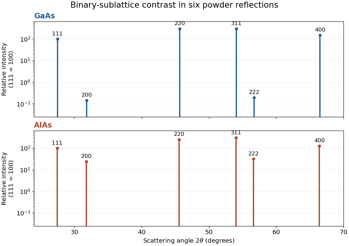
Approximate powder-reflection contrast for GaAs and AlAs
. Original stick patterns use the six derived angles, , and multiplicity times squared structure amplitude. Each compound is normalized to its own reflection. A logarithmic intensity scale reveals the nearly cancelled and GaAs reflections. Geometry and form-factor corrections are omitted deliberately. Details.
The density of states counts one-electron states per energy interval, including both electron spin orientations. It may be a total or a per-volume quantity; must have the matching normalization. The Fermi-Dirac distributionis the occupation probability of such a state. In the fixed-volume free electron model, the integration variable and the density of states do not depend on . The occupation depends explicitly on and implicitly through the chemical potential needed to preserve electron number. Thermal expansion or a changing electronic band structure would require additional effects outside this model.
At , only states within order of the Fermi energy change their occupation. There are order such states, each carrying an excitation energy of order . Thus and the electronic heat capacity is proportional to . Using the supplied coefficient,The shell argument fixes the scaling, not the numerical coefficient; the controlled Sommerfeld expansion fixes that coefficient at fixed electron number. Filled states far below cannot accept arbitrary thermal excitations because of the Pauli exclusion principle.
At fixed volume and particle number, reversible heating obeys . Integrating the electronic heat capacity from zero temperature givesWith no extensive residual ground-state degeneracy, the third law of thermodynamics sets the electronic . ThereforeThe entropy normalization follows that of : total, per volume or per mole. Lattice contributions are additional and are not part of this electronic result.
Let denote the spin-summed density of states per volume. An electron moment with magnitude the Bohr magneton has Zeeman energies . At low temperature, the two spin populations areThe common chemical potential changes only at order , so it does not affect this linear imbalance. The magnetization is . Define SI volume magnetic susceptibility by and take the weak applied field as . Then Pauli paramagnetism givesThe last equality uses the three-dimensional parabolic free electron model, . This susceptibility is nearly independent of temperature for , unlike the Curie law for localized independent moments. The displayed result excludes orbital diamagnetism and interaction enhancements. If susceptibility instead denotes , omit ; confusing that convention with changes the units.
In the one-band electron Hall effect model, , with . The measured Hall coefficient therefore givesA monovalent body-centered cubic lattice has two conduction electrons per conventional unit cell. Thus , andCounting two spin states within the Fermi sphere gives . Using the specified effective mass in the dispersion,There is one mole of conduction electrons per mole of sodium. Its molar density of states at is , givingUsing the volume density of states in c givesThe effective mass changes the dispersion and density of states; the electron Bohr magneton used for the spin coupling retains the bare electron mass. Replacing it by would be an additional, unjustified magnetic-moment assumption. A Hall factor or a multiband metal would also invalidate the simple density inference; the stated calculation uses the requested one-band approximation.
Take two localized spin orientations with moments along the applied magnetic field. This assumes an electron-like spin factor of two. Their energies are , so the one-moment partition function is , with . The thermal mean moment is , and the spin-one-half paramagnetic magnetization isFor , . With the same SI convention and ,This Curie law is a zero-field or weak-field susceptibility. At arbitrary field the differential response is , and saturates at ; extending the linear law to unlimited field would contradict that finite saturation magnetization.
In the Weiss molecular field approximation, the local response obeysLinearize around in the stable phase of paramagnetism. Substitution of a givesHence the Curie–Weiss law and Weiss temperature areFor positive , is the mean-field theory Curie temperature: the zero-magnetization solution becomes unstable there, and below it a spontaneous solution appears. For negative coupling, a negative fitted Weiss temperature indicates predominantly opposing interactions, but this one-uniform-magnetization treatment does not determine an antiferromagnetic ordering pattern or its transition temperature. More generally the fitted Weiss temperature need not equal the observed ordering temperature.
For , the paramagnetic curve is positive for , diverges as , and tends to at high temperature; its inverse is the straight line . The expression is not the stable susceptibility below . For example substituting would predict a negative response around the unstable branch. The nonlinear self-consistency equation must instead be expanded about the appropriate spontaneous magnetization.
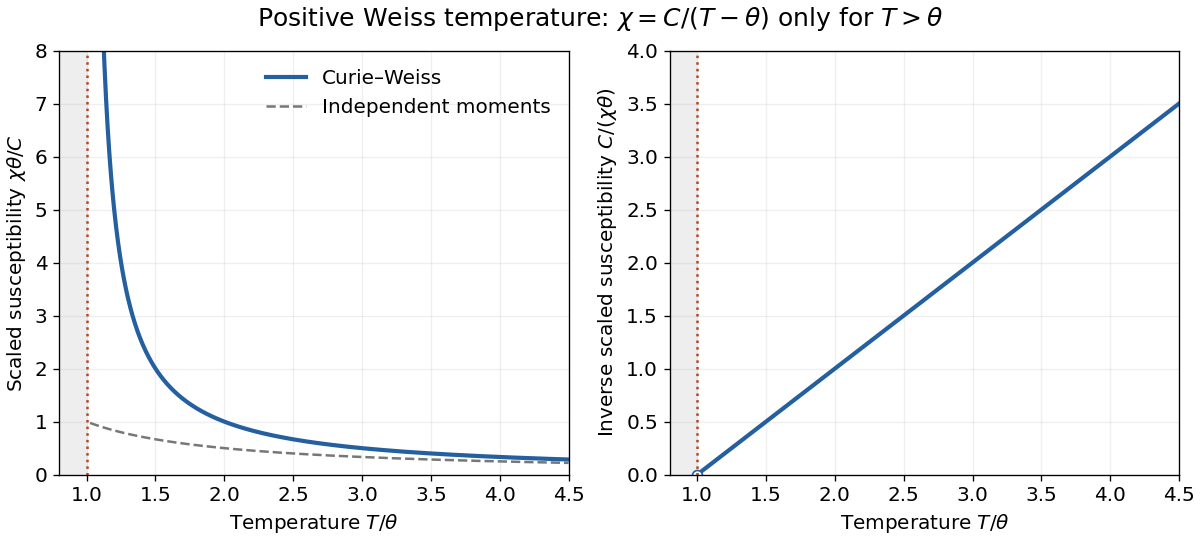
Paramagnetic Curie-Weiss susceptibility and its inverse
. The positive-Weiss-temperature mean-field law is shown only in its stable paramagnetic range . Its inverse extrapolates to zero at . The curve below the transition is not obtained by continuing the displayed rational expression. Details.
Within the stipulated localized, one-moment-per-atom spin model, the number density follows directly from mass density and molar mass:The face-centered cubic lattice is consistent with four atoms per conventional unit cell; no additional factor four is needed once has been obtained from the density. The Curie constant is . Identifying the model's with the specified Curie temperature givesAt very low temperature, a fully ordered single domain has . Its Weiss molecular field isThe cancellation of in the middle expression provides a useful check. The ordinary magnetostatic scale is only , smaller by the factor . Thus is not a plausible ordinary self-generated dipolar magnetic field of the nickel moments. It represents the exchange interaction energy in field units, not an additional Maxwell field of that magnitude. This does not assert that such large externally generated fields are forbidden. Nickel is an itinerant ferromagnet; the imposed one--per-atom model is an estimate rather than its measured microscopic moment.
A macroscopic nickel specimen can split into magnetic domains, each with nonzero local spontaneous magnetization but with different orientations. Their vector contributions can cancel, giving an almost zero measured net magnetization below the Curie temperature. This reduces the external stray-field energy, at the expense of magnetic domain wall energy; the balance favours a multidomain state in many ordinary specimens.
An applied magnetic field can move magnetic domain walls and rotate the domain moments, revealing a large response and eventually saturation magnetization. Thus a zero average does not mean that each local moment has become thermally disordered or that the material is above its Curie temperature. Preparation, shape and domain-wall pinning influence remanence.
Assume thermal equilibrium, a three-dimensional nondegenerate semiconductor, one parabolic conduction extremum and one parabolic valence extremum, with two spin states in each. Use the supplied effective masses as scalar density-of-states parameters. With conduction energy , state counting gives the per-volume density of statesSince , replace the Fermi-Dirac distribution by its Boltzmann factor. Using and the supplied integral,The electron hole occupation is in the valence band. Applying the same integration below givesTheir product cancels the chemical potential, giving the semiconductor mass-action lawThus, for masses expressed in ordinary mass units,The labels in this last box are exponents, unrelated to the magnetic field or Curie constant above. Valley degeneracy or multiple valence bands must be included in the effective density of states, or absorbed into suitable density-of-states effective masses, not counted twice. Real silicon has anisotropic multiple valleys, so its conductivity mass is not automatically its density-of-states mass; the numerical answers below implement the paper's supplied scalar-mass model.[ref]
ECE 340 Lecture 6 by John Dallesasse. Slide 26, A Few Cautions: carrier counting uses the density-of-states effective mass, while silicon conductivity and cyclotron masses differ
The formula is not an identity for arbitrarily degenerate carriers. For a concrete counterexample, take while holes remain dilute. Fermi occupation gives , whereas the Boltzmann replacement would give ; the predicted product then differs by about three orders of magnitude. Separate electron and hole quasi-Fermi levels out of equilibrium would also prevent the cancellation used above.
For an undoped neutral intrinsic semiconductor, . Equating the two expressions from a and taking logarithms givesand hence the intrinsic-semiconductor chemical potentialTherefore . The logarithm is temperature-independent for fixed parabolic effective masses. The chemical potential is exactly at midgap only if the two effective density of states values coincide; for it moves above midgap. Additional valley multiplicities would add their logarithmic contribution.
A substitutional phosphorus atom supplies one more valence electron than the silicon atom it replaces. In the shallow hydrogenic donor state model, the remaining positive impurity attracts that extra electron through the screened Coulomb potentialRescaling the hydrogen atom binding energy by the effective mass and dielectric screening gives the ionization energyThe donor level lies at ; its binding magnitude is positive. The associated effective Bohr radius of a hydrogenic donor is , consistent with a shallow state extended over several lattice spacings.
At , , approximately times this binding energy. Dilute donors are consequently expected to be largely ionized, rather than frozen out. The actual ionized fraction also depends on the chemical potential, available conduction states and donor charge-state degeneracy; comparing to the binding energy alone is not a normalized ionization probability. At sufficiently high temperature, intrinsic electron-hole production can dominate the total carriers even though donors are ionized. Band anisotropy and short-range impurity corrections limit the numerical hydrogenic estimate.
At , . With the scalar effective masses and two-spin convention of a, the effective density of states values areThe intrinsic carrier concentration follows from :From b, . Taking as a reference,It lies above the middle of the band gap, because the hole effective density of states is larger. Both band edges are more than twenty away, validating the nondegenerate semiconductor approximation.
Take uncompensated donor impurities and initially approximate them as ionized. Charge neutrality then gives , while the semiconductor mass-action law gives . Solving the quadratic without prematurely discarding minority carriers,Since , the hole density isUse the conduction population to locate the chemical potential:It moves toward the conduction band but remains about below it, so the mobile electrons are nondegenerate. Despite the donor binding energy being comparable with , the large number of available conduction states makes ionization almost complete at this dilute doping. For a singly occupied two-spin donor, , with . The inferred value is , confirming the approximation to much better than one percent. Including this small correction raises the hole density only to about .
Articles by others on the same topic
There are currently no matching articles.