Original paper: Public original PDF, physical pages 9–16; question pages 10–16.
Use horizontally and vertically, and label each molecular center by its fractional height along the viewing direction. The four centers in one periodic cell are with height and orientation A, with height and orientation A, with height and orientation B, and with height and orientation B. Boundary images complete the projected rectangle. The A and B bonds have opposite slopes; the atoms in each bond are indistinguishable.
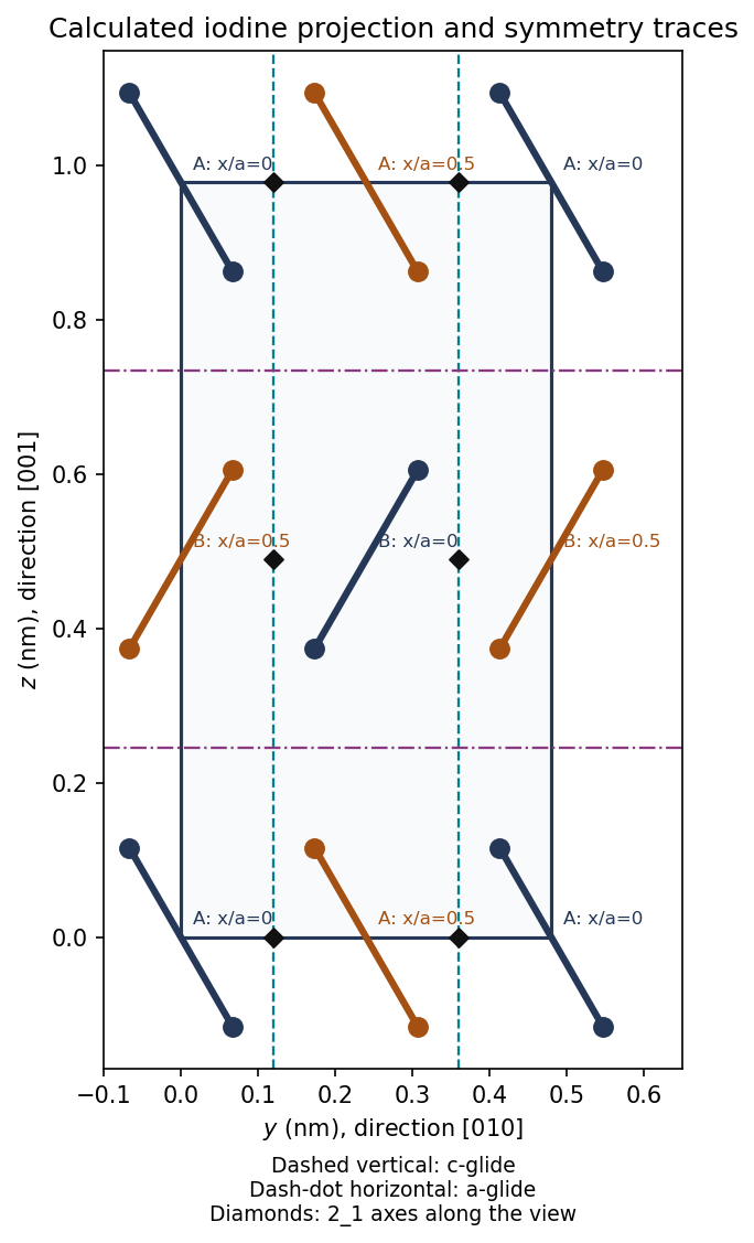
Original molecular-center construction and symmetry traces for the iodine cell viewed along ; bond inclination is schematic, heights and bond length are specified
. Details. 
The height labels matter: a symmetry of the unlabelled projection need not be a translation or reflection symmetry of the three-dimensional crystal. The drawing uses the given molecular bond length and an illustrative inclination, since no exact inclination angle is specified.
This is a C-centered orthorhombic lattice. The translation takes each A molecule to another A molecule and each B molecule to another B molecule. Thus the conventional cell has two lattice points.
A two-molecule crystal motif can be chosen as A at and B at . Attaching that same motif to both C-centered lattice points produces all four molecules, hence eight iodine atoms per conventional cell.
The centers alone appear face-centered, but exchanges A and B orientations. It is not a translation symmetry of the oriented molecular solid. An F-centered assignment would discard essential motif information.
For the first axis the operation in fractional coordinates isIt rotates by about the axis and translates by . For example, it sends the A center at to the A center at , and sends B at to B at modulo integer translations. A half-turn preserves each unoriented diatomic bond. A second application gives one full translation.
There are also ordinary twofold axes through the molecular-center rows; those should not be confused with the screw axes halfway between the corresponding rows.
The relevant planes contain , so their normals lie in the plane. The symmetry operations can be checked directly on the height-labelled molecules:
- Glide planes of type , parallel to at , for example
- Glide planes of type , parallel to at , for example
There are no ordinary mirror planes containing for the illustrated generic bond inclination. Reflection alone would reverse a bond slope without the necessary accompanying translation. A mirror perpendicular to is a different symmetry and is outside the requested zone.
Count atoms before comparing cell volumes. The molecular conventional cell has eight atoms; the metallic face-centered cubic cell has four. ThusRelative to the molecular phase,The transformation therefore produces about 22.2% contraction per atom on the stated extrapolated-volume comparison. Conversely, the molecular volume is about larger than the metallic volume; these percentages have different denominators. Compressibility would be needed to turn the extrapolated comparison into exact volumes at the transformation pressure.
At fixed temperature, a phase's Gibbs free energy satisfies . For the metallic-minus-molecular difference,Increasing pressure favors the smaller-volume metallic phase. With a pressure-independent volume approximation, , so pressure can overcome an initially positive free-energy difference. The volume comparison explains the direction of stabilization; it does not by itself determine the transition pressure or the electronic origin of metallic bonding.
Assume one temperature-independent activation energy over this interval and an unchanged dopant-controlled carrier population. Write the Arrhenius equation as . The two measurements giveUsing yieldsThe Nernst-Einstein relation includes the factor : . For fixed and a fixed correlation correction,Using conductivity proportional to alone would miss the temperature factor. Carrier association, a changing vacancy population or a changing diffusion correlation factor would invalidate this simple extrapolation.
For an oxide ion, or an oxygen vacancy measured relative to the ideal lattice, the charge magnitude is . The independent-carrier Nernst-Einstein inversion at givesHere and must describe the same carrier convention. If the quoted diffusivity is a mobile-vacancy diffusivity, this is the vacancy density. If it is literally an oxygen-ion tracer diffusivity, it is an effective oxygen-ion density under an uncorrelated model. Vacancy density cannot be substituted for oxygen-ion density while retaining the same diffusivity. This distinction is consequential in the last part.
The conventional cubic cell has volumeConsequently the same effective carrier count isA noninteger mean is normal for a doped crystal: it describes an ensemble average, not a requirement that every cell contain the same number of defects. The fluorite structure has four cation sites and eight oxygen sites in this conventional cell.
The numerical vacancy fraction depends on what the supplied diffusivity describes. In the usual effective mobile-vacancy calculation, the carriers per cell are oxygen vacancies, each of effective charge . There are eight oxygen sites, so that convention givesThere is a real qualification: the printed description calls the measured particles oxygen carrier ions. If is their tracer diffusivity and every occupied oxygen site is counted as an uncorrelated carrier, the inversion instead gives , formally . Such an enormous oxygen deficiency is inconsistent with the ordinary lightly doped fluorite picture; it is not a credible deduction of vacancies in stabilized zirconia.
More generally the conductivity involves a collective diffusion coefficient, whereas tracer diffusion includes jump correlations. With the explicitly defined convention ,Without a carrier definition and the relevant correlation information, the literal tracer data do not uniquely establish the vacancy fraction. Thus is a conditional effective-vacancy answer, rather than a convention-free inference. TODO: establish the intended carrier/diffusivity convention if an authoritative clarification becomes available.
Measure ring centers and radii against the printed scale, rather than comparing raw squared radii. A representative reading of the four rings is , with broad photographic lines. For a flat plate at distance ,With the ratios are approximately , givingFor identical atoms at the four conventional FCC positions,The structure factor is for indices all even or all odd, and zero for mixed parity. Thus, for example, 100, 110 and 210 are systematic absences. The allowed squared-index sums begin . Only the first four rings fit within the displayed field; 222 and later allowed reflections are not forbidden merely because they are outside the image. The central shadow and its holder are not extra diffraction peaks.
Take for the unresolved iron doublet. The underlying tabulated and wavelengths are approximately and .[ref]
X-ray wavelengths and X-ray atomic energy levels by J. A. Bearden. Table V, iron entries; physical PDF page17
Using the inferred , Bragg's law gives the following approximate cone angles:The exact angles inherit the lattice-parameter uncertainty. Five reflection families are kinematically possible with this longer wavelength: . The next FCC family, 400, cannot satisfy Bragg's law.
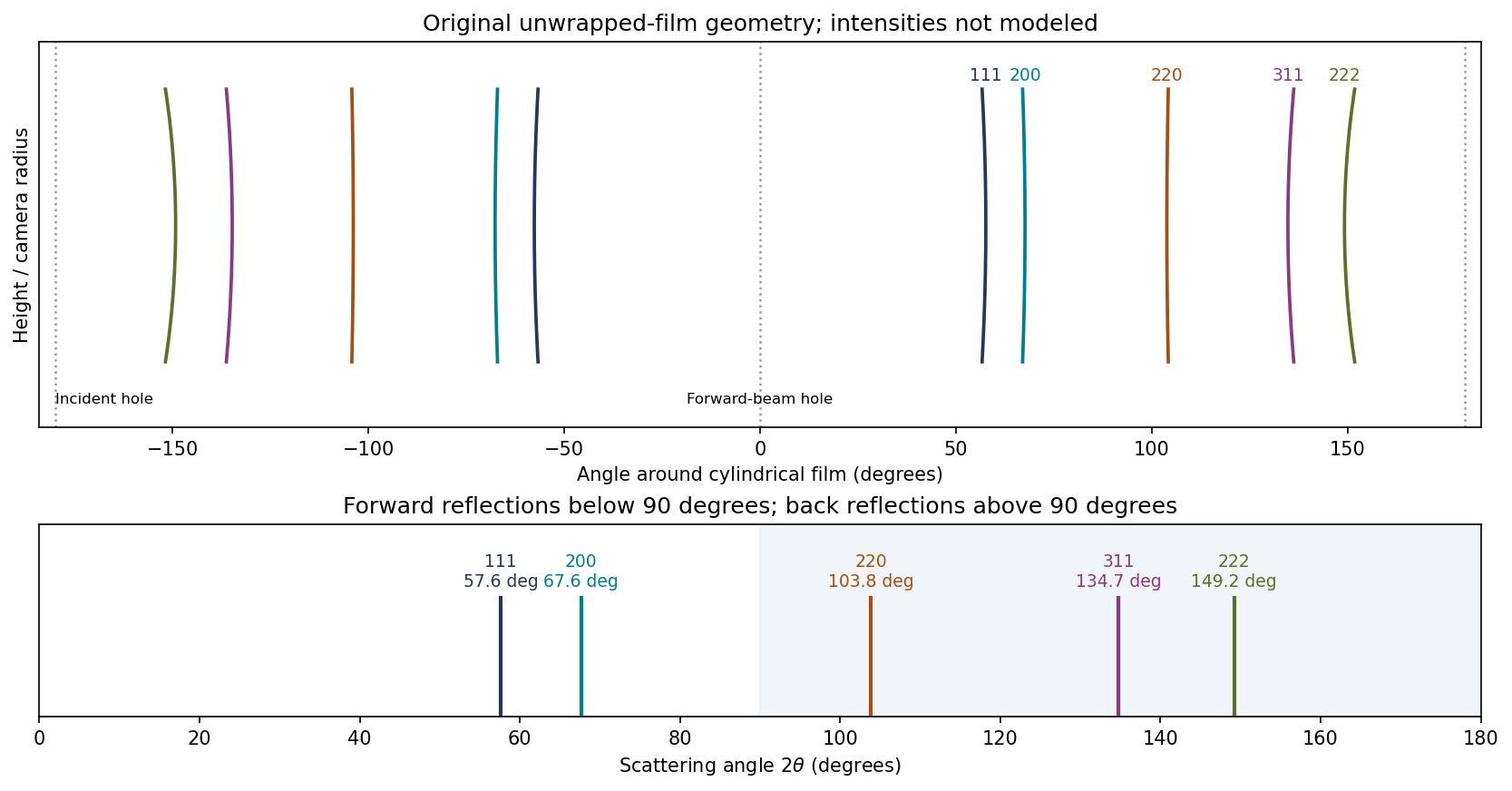
Original calculated Fe cone intersections on unwrapped cylindrical film; angular positions use the measured lattice estimate, line intensities are schematic
. Details. 
A cylindrical Debye-Scherrer camera records paired curved lines where each diffraction cone intersects the film. Both forward and backward cones can be intercepted. The last three families are back reflections here, unlike the rings recorded on the original forward flat plate. Film position is proportional to camera angle along the equatorial circumference, rather than to ; the incident and transmitted beam holes must also be distinguished from reflections. A sufficiently resolved exposure may separate the characteristic doublet, but the schematic does not claim to predict line intensities.
For any indexed cubic reflection,Use for the unresolved molybdenum doublet; the tabulated components are approximately and . These are external spectral constants, not an assertion about the unavailable historical Data Book.[ref]
X-ray wavelengths and X-ray atomic energy levels by J. A. Bearden. Table V, molybdenum entries; physical PDF page19
Reading broad ring centers in the supplied image more closely gives representative radii . Their corresponding estimates are about . Their small scatter understates possible common scale and camera-distance errors. In particular,for a first-order signed perturbation; independent uncertainties are combined in quadrature instead. A reading uncertainty of order , plus the printed-scale and setup uncertainty, justifies a deliberately modest precision:Nickel is a plausible identification, since it is FCC with room-temperature edge about .[ref]
Thermal expansion of nickel and iron, and the influence of nitrogen on the lattice parameter of iron at the Curie temperature by Jinn-Wen Hwang. Abstract, pure-nickel lattice parameter at25°C
The source photograph alone does not chemically identify the specimen; nearby elemental lattice constants and the scale uncertainty preclude a rigorous unique assignment. The estimate is not reported with artificial precision inherited from pixel fitting.Eutectic solidification is the coupled transformation of a liquid into two distinct solid phases at the eutectic temperature and composition, . At fixed pressure in a binary system the three-phase equilibrium is invariant. An exactly eutectic liquid can therefore finish freezing at one temperature, instead of over a broad liquid-plus-solid interval.
Eutectic compositions are useful in joining alloys, for example silver-copper brazing filler: the comparatively low melting temperature and narrow freezing interval help liquid flow into a joint and then solidify. Alternating growth of the two phases often produces a fine lamellar eutectic microstructure. The eutectic is a two-phase aggregate, not a new single solid phase.
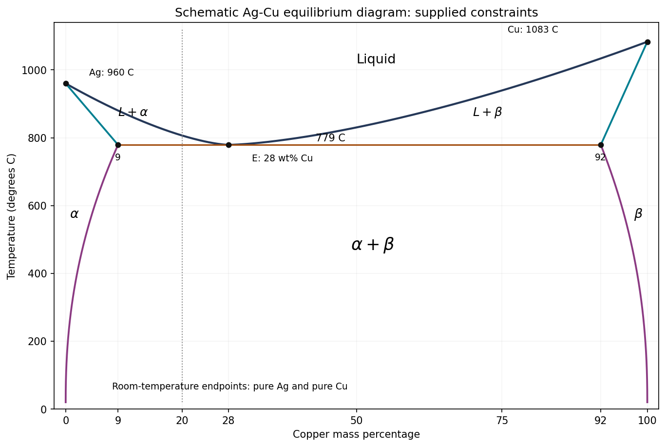
Original schematic Ag-Cu phase diagram constrained by the supplied endpoints and eutectic tie line; unprovided curve shapes and intermediate temperatures are illustrative
. Details. 
The horizontal axis is copper mass percentage. The two liquidus branches meet at and connect to pure silver at and pure copper at . The terminal solid-solution boundaries at the eutectic temperature are Cu for and Cu for . Label the single-phase fields , the two liquid-plus-solid fields , and the lower two-solid field .
The solidus boundaries link the pure-component melting points to their terminal solubility limits; the eutectic isotherm spans the three-phase tie line. Below it, the solvus branches approach pure Ag and pure Cu at room temperature. The supplied data determine this topology and the marked points, not the exact shapes of every boundary. The drawing therefore does not invent a numerical liquidus temperature for an intermediate composition.
Apply the lever rule on the solid tie line. All compositions are copper mass percentages:Thus the equilibrium material is 77.1% and 22.9% by mass just below the eutectic temperature. These are phase fractions; converting them to volume fractions would require densities.
The room-temperature endpoints are pure Ag and pure Cu. Conservation of the total copper mass therefore givesThe answer is 72% silver phase and 28% copper phase by mass. The change from the high-temperature fractions is caused by decreasing solid solubility: the phases reject the opposite component during equilibrium cooling. Simply retaining the eutectic-temperature lever-rule fractions would violate the stipulated room-temperature equilibrium compositions.
The cooling curve first falls in the entirely liquid field. On crossing the liquidus, primary Ag-rich begins to grow. Latent heat release makes the descent shallower; the remaining liquid becomes richer in copper and approaches the eutectic composition.
At , the remaining liquid solidifies as , giving an isothermal arrest under the ideal equilibrium, heat-extraction model. After the liquid is exhausted, temperature falls through the two-solid field. Continued loss of solid solubility causes additional redistribution and precipitation; it does not require another invariant liquid-freezing plateau.
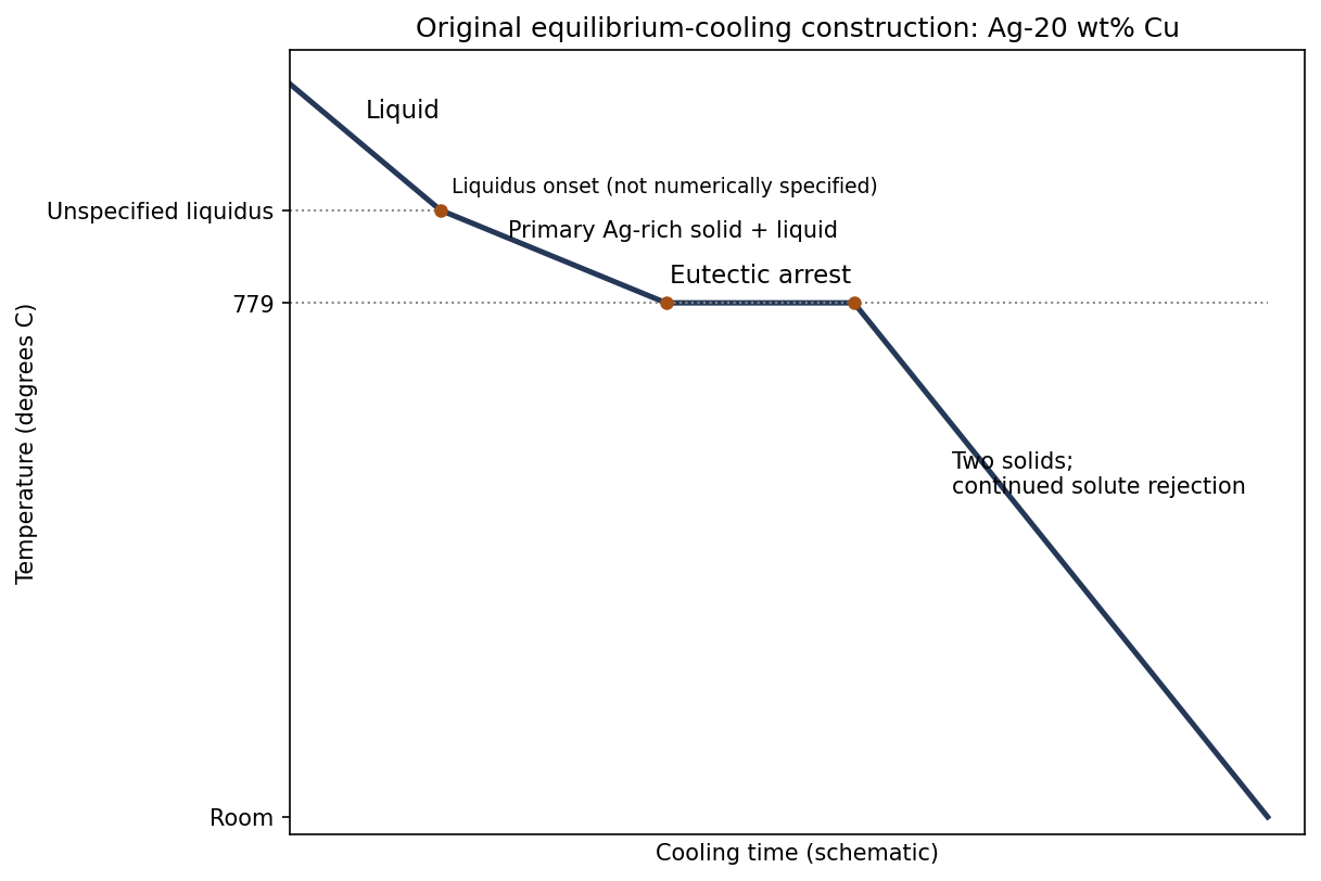
Original schematic cooling curve for Ag-20 wt% Cu, with an unspecified liquidus kink and a labelled eutectic arrest
. Details. 
Immediately before the eutectic reaction, the remaining liquid fraction isThe arrest represents freezing of roughly of the sample by mass. Its duration cannot be calculated without the heat-extraction rate and latent heat, and the onset temperature cannot be calculated exactly from the supplied phase-diagram points alone.
At equilibrium at room temperature the phases are pure Ag and pure Cu, with mass fractions and . A representative solidification structure contains primary Ag-rich grains or dendrites surrounded by a finer two-phase eutectic aggregate. Subsequent equilibrium solute rejection modifies both constituents as they cool.
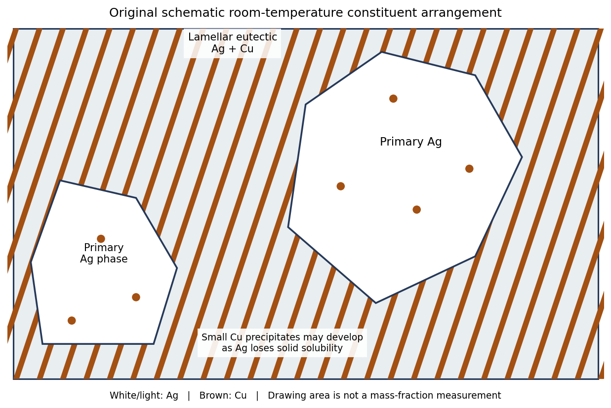
Original schematic primary-silver and lamellar eutectic arrangement; geometrical drawing areas do not assert mass or volume fractions
. Details. 
The primary- and eutectic-constituent fractions calculated at the eutectic arrest describe how the liquid froze. They are not the final pure-Ag and pure-Cu phase fractions. For example, just below the arrest the total copper-rich phase fraction is ; it rises to as solubility is lost on further equilibrium cooling. The distinction separates a microstructural constituent from a thermodynamic phase.
Faster solidification usually refines the dendrite and eutectic spacings. If solid-state diffusion cannot keep up, composition gradients, supersaturated solids and delayed precipitation can persist. Their exact fractions then depend on the thermal history; faster cooling does not change the alloy's overall copper inventory. Complete long-term equilibration would restore the same equilibrium phase compositions and mass fractions.
The alloy shear yield stress can be roughly times the stated pure-aluminium critical resolved shear stress. Strengthening raises the stress required for dislocation glide rather than requiring homogeneous shearing of a perfect crystal.
- Solid-solution strengthening: substitutional solutes create elastic and chemical disturbances that interact with dislocations. A moving dislocation must escape or drag these disturbances.
- Precipitation hardening: suitably spaced second-phase particles obstruct glide. Small shearable precipitates resist cutting; larger nonshearable obstacles require dislocation bowing and bypass. Particle spacing and coherency matter, so overaging can reduce strength.
- Work hardening: prior plastic deformation increases dislocation density. Intersections, junctions and forest dislocations impede subsequent glide; a common scaling is .
- Grain boundary strengthening: smaller grains shorten the distance over which dislocations can pile up and make slip transfer across differently oriented grains more difficult. In its ordinary regime, the Hall-Petch relation is .
These mechanisms can coexist. The numerical comparison is an order-of-magnitude comparison of shear strengths; it is not a conversion of the alloy's shear yield stress directly into a tensile yield stress.
For a coarse-grained, approximately untextured polycrystal undergoing general plastic flow, use the conventional orientation-and-compatibility estimateWith the supplied ,The round result is a conventional estimate for an unspecified coarse polycrystal, not a material-independent exact conversion. The most favorably oriented individual grains can first slip at ; that is not the same event as compatible macroscopic yielding throughout the aggregate.
There is no single crystallographic tensile axis for all grains. Individual grains rotate and can develop crystallographic texture, while the macroscopic bar remains loaded along its tensile axis. A specified initial texture or yield criterion would be needed for a more exact numerical prediction.
For FCC aluminium, consider slip. Normalize the tensile direction and one candidate system:Here . Comparing all twelve systems gives the largest Schmid factor on :Schmid's law therefore givesDuring ideal single slip, the tensile direction expressed in crystal coordinates rotates towards , along the great-circle path joining the original axis to that slip direction. It reaches a symmetry boundary where another slip system becomes equally favored. This single-slip tensile-axis rotation concerns the crystal relative to the externally held loading direction, rather than a rotation of the laboratory loading apparatus.
Take ordinary basal slip in magnesium, . In three-index hexagonal notation, denotes a vector proportional to , not a cubic Cartesian with equal axis lengths. The basal slip direction closest to the tensile axis is along ; its four-index representative is .
For ,Thus the algebraic answer isAn external crystallographic reference gives and , hence and . This is a conditional external-data estimate, not a fabricated value attributed to the supplied Data Book.[ref]
Crystal Structures by R. W. G. Wyckoff. Volume1, magnesium entry reproduced in COD9008506
The tensile axis rotates towards the selected basal slip direction during ideal single slip. As the axis approaches the basal plane, the resolved basal shear eventually becomes small; other modes, hardening and instability can interrupt the single-slip description. TODO: verify the exact magnesium lattice ratio supplied in the historical examination Data Book. Taking a angle solely from the indices would incorrectly use a cubic metric.
A second slip system begins to operate as the tensile-axis rotation makes its resolved shear stress comparable to that on the primary system. Dislocations on intersecting planes interact much more strongly, giving the transition from easy single slip to rapid work hardening. The standard geometric estimate neglects differences between the evolving critical stresses of the two systems.
The primary direction is . Single-slip shear carries the line joining the specimen ends, expressed in crystal coordinates, alongThe initial fundamental sector has . Its first reached boundary is , at , giving . At that orientation and have equal Schmid factors. Since the component perpendicular to the primary slip direction is unchanged by that shear, the length ratio follows directly:ThereforeThe corresponding logarithmic strain is . This is an ideal equal-critical-stress geometric onset estimate. Real secondary slip can start earlier or later because of latent hardening, nonuniform deformation and grip constraints; the problem supplies no hardening law that would determine that shift.[ref]
Applied Mechanics of Solids by A. F. Bower. §3.12.2, points10–12: tensile-axis rotation, secondary slip and stages of hardening
The printed numerical ratios are about , not about :The qualitative contrast is nevertheless meaningful. FCC aluminium has close-packed glide planes and relatively mobile dislocations. Magnesium also has easy close-packed basal glide, although it lacks enough equivalently easy slip systems for arbitrary room-temperature polycrystal deformation.
BCC iron has no close-packed plane. Its screw-dislocation cores and lattice-friction barrier give much stronger resistance to glide; thermally activated kink motion makes the critical stress particularly temperature- and rate-sensitive. This is the relevant Peierls-stress explanation. A high polycrystal constraint factor cannot explain the supplied contrast, because the data are already critical resolved shear stresses. Neither the precise factor35 nor a universal BCC/FCC ratio follows from crystal packing alone: purity, dislocation structure, temperature and testing conditions also matter.
For a spherical homogeneous nucleus, the capillarity approximation givesThe first term penalizes creating an interface; below the melting point the bulk free-energy change per volume is negative and favors growth. Near , neglect the temperature dependence of the latent heat. Since the free-energy difference vanishes at ,Set the radius derivative to zero:The nonzero stationary point is a maximum, since . Subcritical nuclei lower free energy by shrinking; supercritical nuclei lower it by growing. The positive radius and its inverse-supercooling dependence follow from the negative freezing enthalpy. This derivation assumes an isotropic, size-independent interfacial energy and a bulk-like spherical nucleus; it is not a molecular-scale kinetic theory.
TODO: user-deferred biology. No biological nucleation-agent calculation or biological interpretation has been researched or supplied.
TODO: user-deferred biology. No organism-specific survival mechanism has been researched or supplied.
TODO: user-deferred biology. No organism-specific survival mechanism has been researched or supplied.
TODO: user-deferred biology. No organism-specific survival mechanism has been researched or supplied.
Material creep is time-dependent permanent deformation under sustained stress. Its rate is often appreciable at a large homologous temperature , because diffusion and obstacle-escape processes become rapid. In an activated regime a useful form iswith additional elastic, geometric and temperature prefactors absorbed into for the chosen approximation. The activation energy belongs to the rate-controlling process: bulk diffusion, grain-boundary diffusion and dislocation motion need not have the same value.
- A: power-law dislocation material creep. Dislocations glide and climb around obstacles; vacancy transport enables climb and recovery. The rate is strongly stress-dependent, typically with several times greater than one. It dominates the higher-stress, hot field below the glide-strength boundary.
- B: Nabarro-Herring creep. Stress-directed vacancy diffusion through the grain interiors transfers material between differently stressed boundaries, extending grains along tension. In the simple equiaxed-grain model . It occupies the high-temperature, low-stress field.
- C: Coble creep. The analogous transport runs predominantly along grain boundaries. The characteristic scaling is , where is an effective boundary thickness. The lower activation cost of boundary diffusion makes it competitive at lower temperature than bulk-diffusion material creep.
Boundary sliding can accommodate grain-shape changes during diffusional material creep; it is not a reason to identify either diffusion field as dislocation glide. The supplied map's A/B/C placement, including the boundary between B and C, determines these assignments. Its numerical contours apply to the material state used to construct that map, not to arbitrary grain sizes.
Lower the operating temperature or stress, suppress diffusion, and remove or stabilize the paths that accommodate material creep. Increasing the melting temperature can reduce at a specified operating temperature. Chemistry that reduces diffusivity or impedes dislocation climb can reduce the material creep rate; stable precipitates or dispersoids can resist glide and climb, provided they do not dissolve or coarsen rapidly in service.
Large grains reduce both Nabarro-Herring and Coble creep, according to their and dependencies. Directional solidification can reduce boundaries normal to the dominant tensile stress, while a single crystal removes grain-boundary transport and sliding from the ordinary polycrystal mechanism inventory. It does not remove bulk diffusion or dislocation material creep.
This is why room-temperature grain-refinement strengthening is not automatically a high-temperature material creep strategy: fine grains create more boundary transport paths. Any protective microstructure must remain stable at the service temperature, and the design must also avoid stress concentrations and unwanted thermal loading.
At height above the free lower end, a uniform vertical filament carries the weight of length . With cross-sectional area ,The maximum stress is at the top and is independent of diameter. The diameter cancels because both mass and load-bearing area scale with . Neglecting self-heating gradients, evaporation and initial fabrication stress, this top point sets the first creep-strain limit.
For a clearly labelled external reference estimate, take . Then ; the area is and the total suspended mass is about . The density is independently tabulated, not invented as a supplied 2016 value.[ref]
Atomic and nuclear properties of tungsten by the Particle Data Group. 2009 table, density entry
Use the original map's top temperature axis at and its right-hand tensile-stress axis, so no uncertain shear-stress conversion or additional shear modulus is required. The point lies in C, between the and contours, nearer . A logarithmic interpolation of the scanned contours gives about , with only graphical precision. Thusor of order three months in this steady-rate, reference-density map estimate. Reading only the bracketing contours gives the appropriately broad interval to ; the graph does not support an exact service-life number.
For the exact prescribed input, the answer remainsTODO: verify the density convention in the historical Data Book and the applicability of the supplied map to the filament's grain structure. Thermal expansion lowers density, and an evolved area or tertiary material creep changes the rate; a steady initial-rate estimate is not a guaranteed lifetime. In particular, the source map has its own fixed grain-size assumptions and no separately specified filament grain size. Other failure mechanisms could shorten useful life.
Articles by others on the same topic
There are currently no matching articles.