Past exam of the mathematical methods II course of the University of Oxford / 2013 (4296, CP4)

Source: public Oxford archive. The held cover dates this ordinary sitting to 6 June 2013. All four Section B options are answered.

Work where $x\ne 0$ and $f$ is differentiable. Set $q=y/x$. The chain rule givesConsequentlyGeometrically, a radial rescaling of both coordinates leaves $y/x$ unchanged, so the function has zero rate of change along radial dilations. No value or derivative at $x=0$ is implied by this representation.

Put $h=x-\pi /2$. Periodicity gives $\tan (2x)=\tan (\pi +2h)=\tan (2h)$. The local Taylor expansion $\tan (2h)=2h+O(h^3)$ therefore yieldsAlthough $\tan x$ is singular at $\pi /2$, the numerator here is $\tan (2x)$, which is smooth and zero there.

Continuity at $x=2$ requires both one-sided limits to equal the specified value $3$. The right branch gives $a+2b=3$ and the left branch gives $b-4a=3$. Solving these two linear equations givesSubstitution gives $-1/3+10/3=3$ on the right and $5/3+4/3=3$ on the left. These conditions enforce continuity, without requiring the two one-sided derivatives to agree.

For $\mathbf{r}(t)=(t,t^2,t^3)$, the endpoints correspond to $t=0,1$ and $\dot{\mathbf{r}}=(1,2t,3t^2)$. The vector field on the path is $\mathbf{A}=(9t^2,-14t^5,20t^7)$, so the line integral isIncluding the derivative of each path coordinate is essential; merely substituting the path into the field does not supply the line element.

Parametrize the straight path by $\mathbf{r}(t)=(t,t,t)$ for $0\le t\le 1$. Then $\dot{\mathbf{r}}=(1,1,1)$ and $\mathbf{A}=(3t^2+6t,-14t^2,20t^3)$. ThusThis differs from the preceding path's value. Indeed, $\nabla \times \mathbf{A}=(14y,-20z^2,-6)$ is not zero, so the field is not a conservative vector field and its integral need not depend only on endpoints.

The gradient is $\nabla T=2(x,y)/(x^2+y^2)$ and at $(1,2)$ it is $(2/5,4/5)$. The directional derivative along a unit vector is maximal in the gradient direction. ThereforeThe direction is radially outward from the origin, perpendicular to the circular level curve through the point.

Let $s\ge 0$ be distance along the unit direction from part (a). The point is $\mathbf{r}(s)=(1,2)+s(1,2)/\sqrt{5}$, whose distance from the origin is $\sqrt{5}+s$. For finite increments of a logarithmic radial function, the exact change isThus an increase of $0.2$ requiresIf the intended calculation is the local directional derivative estimate, its first-order value is $s\simeq \Delta T/|\nabla T|=\boxed{\sqrt{5}/10}$. The latter approximates the exact finite distance rather than equaling it. Numerically they are about $0.235$ and $0.224$, respectively.

Normalize the specified direction to $\hat{\mathbf{u}}=(1,1)/\sqrt{2}$. At distance $s\ge 0$ the squared radius is $(1+s/\sqrt{2}{)}^2+(2+s/\sqrt{2}{)}^2=5+3\sqrt{2}s+s^2$. The exact change $\Delta T=0.12$ therefore requires $5+3\sqrt{2}s+s^2=5e^{0.12}$. The positive root isFor comparison, the initial directional derivative is $(2/5,4/5)\cdot (1,1)/\sqrt{2}=3\sqrt{2}/5$. Its first-order distance estimate isThese give approximately $0.145$ and $0.141$. The exact expression accounts for the changing gradient along a finite straight displacement.

A stationary direction at the point has zero directional derivative, hence is perpendicular to $(1,2)$. The two opposite unit directions areThey are tangents to the circular level curve. “Stationary” here means zero first-order change. A finite straight move in a tangent direction gives squared radius $5+s^2$ and therefore a positive second-order change $\ln (1+s^2/5)$; following the curved level set instead keeps $T$ exactly constant.

The cardioid has nonnegative polar radius $r=1-\cos \theta$, ranging from zero at the right-hand cusp to two on the negative $x$ axis. Its intersections with the circle $r=3/2$ satisfy $\cos \theta =-1/2$, giving $\theta =2\pi /3,4\pi /3$. The selected region is the left-hand cap between the two curves:The endpoints in Cartesian coordinates are $(-3/4,\pm 3\sqrt{3}/4)$.

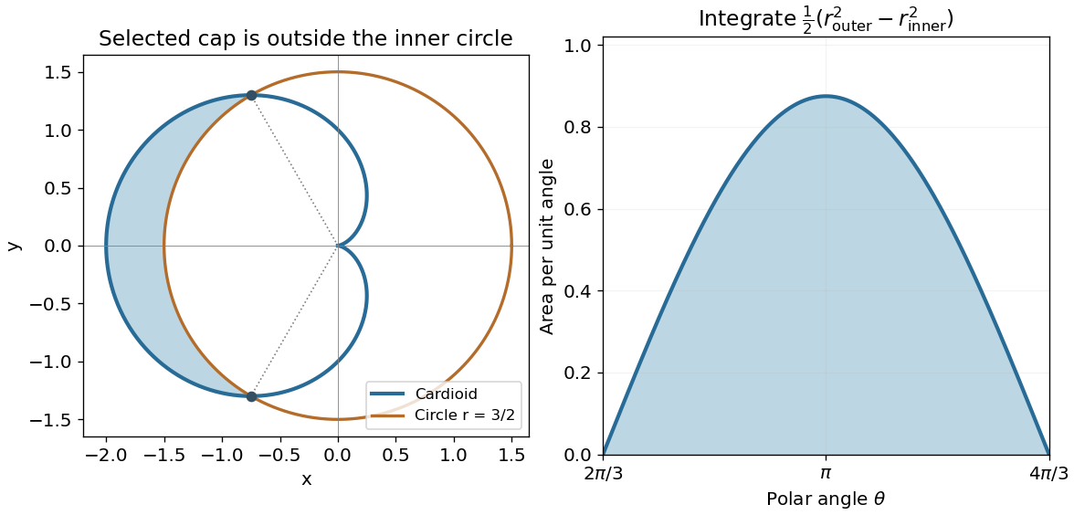
In polar coordinates, the area element is $rdrd\theta$. Using the bounds from part (a),Since the bracket equals $-3/4-2\cos \theta +(1/2)\cos 2\theta$, an antiderivative is $-3\theta /4-2\sin \theta +(1/4)\sin 2\theta$. Evaluation givesThe inner-circle contribution must be subtracted before angular integration; integrating the entire cardioid or the entire circle would include regions excluded by the specified intersection.

The change of variables has inverse $x=(u+3v)/7$, $y=(v-2u)/7$, with absolute inverse Jacobian determinant $1/7$. The two lines $y=-2x+1,-2x+4$ become $v=1,4$, and $y=x/3,(x-7)/3$ become $u=0,7$. Hence the parallelogram maps to a rectangle andThe denominator $v$ is bounded away from zero throughout the rectangle, so this transformation introduces no improper-integral issue.

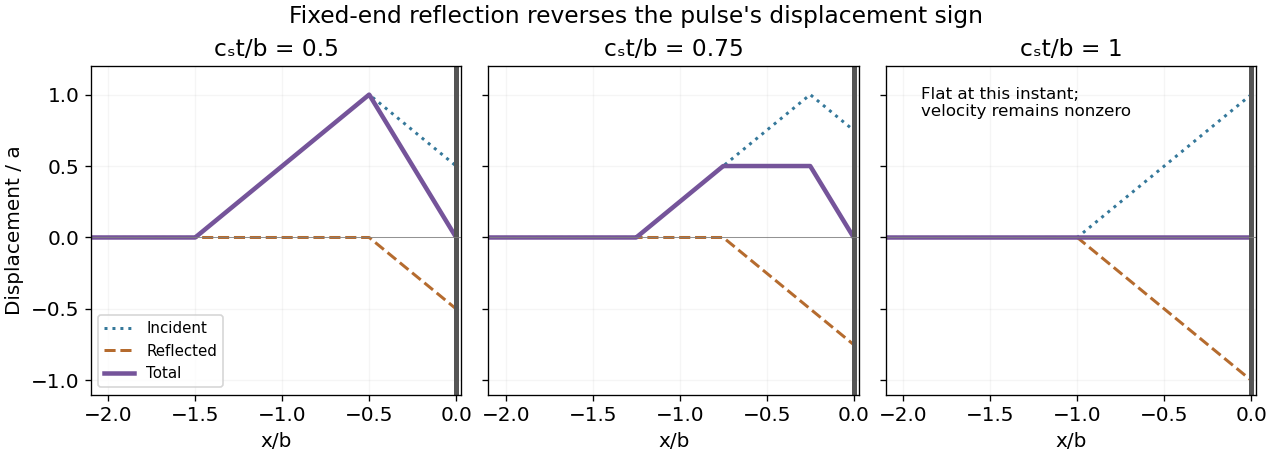
Let $f(x)$ be the initial triangular profile, extended by zero for $x>0$. For fixed-end reflection of a triangular pulse, the right-moving incident component is $f(x-c_{s}t)$; the reflected pulse at a fixed end has opposite sign. The full solution on $x\le 0$ isIt satisfies $y(0,t)=0$ exactly. Write $\xi =x/b\le 0$ and measure displacement in units of $a$, assuming $a,b,c_s>0$. At the first specified time the profile isAt the second time it isAt the third time the two components cancel throughout the half-string:This flat instantaneous profile does not mean the wave energy has vanished. On $-b<x<0$, its velocity at $t_3$ is $-2a{c}_s/b$, and it subsequently becomes a negative reflected pulse travelling left.

With angles measured from the downward vertical, the upper mass rises by $2l(1-\cos {\theta }_1)$ and the lower by $2l(1-\cos {\theta }_1)+l(1-\cos {\theta }_2)$. Taking zero gravitational potential energy at the hanging equilibrium therefore gives the exact resultBoth masses contribute to the elevation change caused by the upper rod.

Use positions ${\mathbf{r}}_1=(2l\sin {\theta }_1,-2l\cos {\theta }_1)$ and ${\mathbf{r}}_2={\mathbf{r}}_1+(l\sin {\theta }_2,-l\cos {\theta }_2)$. Their squared speeds are $4l^2{\dot{\theta }}_1^2$ and $4l^2{\dot{\theta }}_1^2+l^2{\dot{\theta }}_2^2+4l^2{\dot{\theta }}_1{\dot{\theta }}_2\cos ({\theta }_1-{\theta }_2)$. Summing their kinetic energies givesNo small-angle approximation has been used here.

Retain terms quadratic in the small displacements and velocities. The approximations $1-\cos \theta \simeq {\theta }^2/2$ and $\cos ({\theta }_1-{\theta }_2)\simeq 1$ yieldThus the correct quadratic forms areSource correction. The printed kinetic-energy matrix formula omits both time-derivative dots. It cannot hold as a function of angles alone: at $\mathbf{\theta }=0$, ${\dot{\theta }}_1\ne 0$, ${\dot{\theta }}_2=0$, the actual kinetic energy is $4m{l}^2{\dot{\theta }}_1^2>0$, whereas the printed undifferentiated quadratic form vanishes.

For the constant small-oscillation matrices, the total mechanical energy satisfiesThe specified conservative pendulum has Lagrangian $L=K-U$, whose Euler-Lagrange equations giveor $8{\ddot{\theta }}_1+2{\ddot{\theta }}_2+(4g/l){\theta }_1=0$ and $2{\ddot{\theta }}_1+{\ddot{\theta }}_2+(g/l){\theta }_2=0$. These equations make $\dot{E}=0$.

The scalar energy law alone is insufficient to infer two unique equations: energy conservation does not uniquely determine equations of motion. In particular, adding $\mathbf{G}\dot{\mathbf{\theta }}$ on the right with antisymmetric $\mathbf{G}$ changes the dynamics but contributes zero power. The conservative-force structure of the given pendulum excludes that extra gyroscopic force and supplies the information needed for the displayed matrix equations.

For $\mathbf{\theta }=\mathbf{a}\cos (\omega t+\phi )$, a nonzero normal mode satisfies $(\mathbf{V}-{\omega }^2\mathbf{T})\mathbf{a}=0$. With $s={\omega }^{2}l/g$, its determinant is $4(s^2-3s+1)$. Hence the normal modes of a double pendulum with a two-to-one length ratio haveThe slow mode is in phase and the fast mode out of phase. The general small motion is their superposition with independent amplitudes and phases; ordinary frequencies are ${\omega }_{\pm }/(2\pi )$.

Assume the stated continuous derivatives on an open simply connected region. If $N_x-M_y=0$, Green's theorem gives zero circulation around every simple closed curve and its enclosed region; a piecewise smooth closed curve can be decomposed into such loops, giving the same conclusion.

Conversely, suppose every closed-curve integral vanishes. Apply Green's theorem to an arbitrarily small disk about any interior point $P$. Its integral of $N_x-M_y$ is zero. Divide by the disk area and shrink its radius to zero; continuity makes the average approach $(N_x-M_y)(P)$, so that value must vanish. ThusSimple connectivity is needed for the global sufficiency statement, ensuring that a loop does not enclose a missing portion of the domain. Local necessity already follows from small disks.

On the punctured plane $x^2+y^2>0$, write $M=-y/(x^2+y^2)$, $N=x/(x^2+y^2)$. Direct differentiation givesThere is no $z$ dependence or $z$ component, soThe origin is excluded: the field is undefined there. A zero classical curl away from the origin does not state that the field is smooth on an entire disk containing it.

Along a path avoiding the origin, polar coordinates givewhere the angle is followed continuously along the path. For a closed path its total change is an integer number of turns, soFor a simple counterclockwise loop, the value is $2\pi$ if the origin lies inside and zero if it lies outside. Clockwise orientation reverses the nonzero sign. The winding number formula also handles repeated or self-intersecting loops. A curve passing through the origin is outside the ordinary line integral's domain.

There is no contradiction. The domain on which the field is smooth is the punctured plane, which is not simply connected. A loop enclosing the origin cannot be spanned by a planar region entirely inside that domain, so the smoothness hypothesis needed to apply Green's theorem to its full interior fails. A loop that bounds a region avoiding the origin does have zero circulation.

Locally the field is the gradient of the polar angle, but that angle cannot be made a single-valued continuous potential on the whole punctured plane. The nonzero period $2\pi$ around the hole measures this global obstruction, despite the field having zero local curl.

The terms $u_{tt}$ and $c^2{u}_{xx}$ must have the same dimensions. Likewise $au$ must match $u_{tt}$. ThusOnly $c^2$ occurs in the equation, so its characteristic speed is $|c|$ when $c\ne 0$.

For a nonzero plane-wave amplitude, substituting $u=A{e}^{i(kx-\omega t+{\theta }_0)}$ gives $u_{tt}=-{\omega }^{2}u$ and $u_{xx}=-k^{2}u$. ThereforeThis dispersion relation is not proportionality between frequency and wavenumber: for $a>0$, the phase speed depends on $k$. Thus a superposition generally experiences dispersion. The negative-frequency branch is its opposite; $A=0$ is the trivial solution and imposes no constraint on the unused phase parameters.

The real part $A\cos (kx-\omega t+{\theta }_0)$ represents a monochromatic travelling wave for $k\ne 0$. The magnitude $|A|$ is its displacement or field amplitude, and $\theta =kx-\omega t+{\theta }_0$ is its phase, with ${\theta }_0$ an initial phase offset. The complex exponential is a convenient representation of that real oscillation.

Following a constant-phase point gives $kdx/dt-\omega =0$, soOn the positive-frequency, positive-$k$ branch,For negative $k$, $\omega /k$ is negative on that frequency branch and encodes the reversed direction. At $k=0$, the mode is spatially uniform with frequency $\sqrt{a}$, so a propagation phase speed is not defined.

Differentiate the positive-frequency dispersion relation with respect to $k$:Where $k\ne 0$, $c_p{c}_g=c^2$. For $a>0$ and $c\ne 0$, the magnitude of the group velocity is below $|c|$ even though the positive-$k$ phase velocity exceeds $|c|$. At $k=0$, the group velocity is zero. The two velocities describe envelope and phase transport, respectively.

A local-wave description requires an identifiable smooth phase $\Theta (x,t)$ with $\bar{k}={\Theta }_x$ and $\bar{\omega }=-{\Theta }_t$. Real propagating wavenumber and frequency must satisfy the chosen local branch of ${\bar{\omega }}^2=c^2{\bar{k}}^2+a$. In a geometrical optics or slowly modulated wavepacket approximation, these quantities and the amplitude vary on scales large compared with a local wavelength and period; for example $|{\partial }_x\bar{k}|\ll {\bar{k}}^2$ and $|{\partial }_t\bar{\omega }|\ll {\bar{\omega }}^2$ away from degenerate points.

The phase compatibility in geometrical optics means the local fields cannot be specified independently: equality of mixed phase derivatives requires ${\bar{k}}_t+{\bar{\omega }}_x=0$, derived as wave conservation below. These phase and scale conditions justify the local dispersion relation; they alone are not a guarantee of an arbitrary-amplitude exact PDE solution. Amplitude transport and higher-order envelope terms must also be satisfied.

On a locally right-moving branch with $\bar{k},\bar{\omega }>0$, a spatial phase increase of $2\pi$ counts one wave. The local number of waves per unit length and the number passing a fixed point per unit time areThe physical unsigned counts use absolute values on other branches; the signed phase convention is useful for the conservation law. A phase change around a small spacetime rectangle must close. Equivalently, ${\bar{k}}_t={\Theta }_{xt}$ and ${\bar{\omega }}_x=-{\Theta }_{tx}$, soThis wave conservation equation states that the wave count in an interval changes by the crest flux through its ends, provided the smooth phase description has no defects or creation of crests inside. It is phase compatibility, distinct from energy conservation or wave-action conservation.

For a medium with constant coefficients, $\bar{\omega }=\omega (\bar{k})$ on the selected branch. The spatial chain rule gives ${\bar{\omega }}_x=(d\omega /dk{)}_{\bar{k}}{\bar{k}}_x=c_g(\bar{k}){\bar{k}}_x$. Thus wave conservation becomesAlong a characteristic curve with $dx/dt=c_g(\bar{k})$, the total derivative $d\bar{k}/dt$ vanishes. A slowly varying wavenumber feature, and hence the corresponding modulation of a narrow-band packet, travels with the group velocity rather than the carrier's phase velocity. This interpretation assumes the modulation remains smooth on the scale required in part (e).

Let $\mathbf{r}(s)$ be any smooth curve in the level surface $\varphi =c$. Differentiating the constant value along it givesThe curve tangent can be any tangent vector to a regular level set, soThe nonzero-gradient condition matters for determining a normal direction. For example, $\varphi =z^3$ has the plane $z=0$ as a level set, but its gradient vanishes there and supplies no direction, even though the geometric plane has a well-defined normal.

Use the ambient position coordinates $\mathbf{r}$ and a fixed point $\mathbf{a}$. The distance is $R=|\mathbf{r}-\mathbf{a}|$, so $R^2=(x-a_x{)}^2+(y-a_y{)}^2+(z-a_z{)}^2$. Taking its gradient gives $2R\nabla R=2(\mathbf{r}-\mathbf{a})$. Therefore, away from $P=A$,It points from $A$ to $P$. The gradient is taken in the surrounding space and then evaluated on the surface; the intrinsic surface gradient of restricted distance would instead be its tangential projection and need not have unit magnitude.

For reflection between the foci of an ellipse, assume $s>|A-B|$ and define $\Phi (P)=R_A(P)+R_B(P)$. From part (b),On the ellipse this sum is normal to the tangent. Thus a unit tangent $\mathbf{\tau }$ obeys $\mathbf{\tau }\cdot {\mathbf{u}}_A=-\mathbf{\tau }\cdot {\mathbf{u}}_B$. The magnitudes of the projections of the two unit focal directions on the tangent are equal, provingfor the corresponding acute, unoriented line angles.

More explicitly, let $\mathbf{n}=({\mathbf{u}}_A+{\mathbf{u}}_B)/|{\mathbf{u}}_A+{\mathbf{u}}_B|$. The law of reflection maps an incoming unit ray ${\mathbf{u}}_A$ towhich points from $P$ toward $B$. Thus the equal-angle property has the correct incoming/outgoing ray orientation, rather than merely an algebraic bisector assertion.

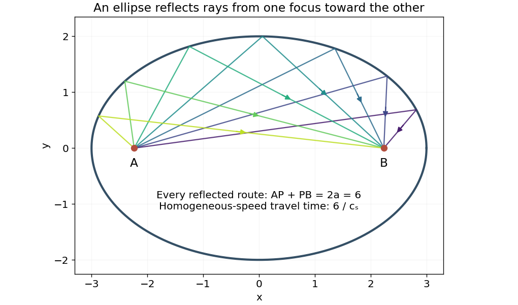
In a homogeneous medium and the short-wavelength ray approximation, a smooth reflecting elliptical boundary sends a ray from focus $A$ to focus $B$ after one specular reflection, by the equal-angle property just proved. Moreover, every such route has the same path length $AP+PB=s$, hence the same propagation time $s/c_s$ for constant sound speed $c_s$.

An ideal two-dimensional elliptical reflector, or the corresponding ellipsoidal geometry, therefore concentrates sound near the other focus; equal travel times also support coherent arrival for a monochromatic source with a consistent reflection phase. Finite wavelength, imperfect surfaces, absorption and three-dimensional room geometry limit the focusing. The result predicts a finite physical focal region, not an infinite intensity at a mathematical point.