A norm on a real vector space is a map satisfying exactly when , for real , and . Its induced metric is . The three axioms respectively give definiteness, compatibility with scaling, and the triangle inequality.
Here equivalent metrics means that the two metrics induce the same topology, and Lipschitz equivalent norms means that there are constants such that for every .
Suppose first that the inequalities hold. Since they also hold for , the identity maps between the two metric spaces are Lipschitz continuous. In particular, each is continuous, so the topologies agree.
Conversely, equality of the topologies makes the identity from the -norm to the -norm continuous at zero. There is therefore such that implies . For nonzero , apply this to and use the absolute homogeneity of both norms:The reverse identity is also continuous, so there is with . Rescaling again gives . ThusThe inequalities also hold at zero. This is topology determines norm equivalence; it works in arbitrary dimension because the rescaling argument needs neither a basis nor compactness of a unit sphere.
Expand using the bilinearity and symmetry of the real inner product:Addition proves the parallelogram law,For the maximum norm on , take and . All four vectors have maximum norm one. The left side of the parallelogram law is then , whereas the right side is . The maximum norm cannot come from an inner product.
Use separation of variables in Laplace's equation: writing givesSingle-valuedness requires -periodicity, so the nonconstant angular Fourier modes have integer and are . Their radial solutions are . The zero angular mode has radial solutions . These give the harmonic Fourier expansions in planar concentric domains used below.
For the annulus with , constant boundary data suggest a radial harmonic function . Enforcing both boundary values givesThis has the required boundary values and satisfies . It is unique: the difference of two continuous solutions is harmonic in the annulus and zero on both boundary circles, so the maximum principle for harmonic functions, applied to the difference and its negative, makes it zero.
Regularity at excludes every negative radial power and the logarithmic zero mode. Thus the general regular single-valued harmonic function on the disk has the formThe coefficients must give a series converging locally in the disk; if finiteness and continuity on its boundary are required, the boundary Fourier series must represent the prescribed finite continuous boundary values. Conversely every such locally convergent expansion is harmonic, and the Fourier coefficients on circles show that it includes every regular solution. There is no angular term linear in , because it would be multivalued.
With the usual exterior-boundary interpretation that the harmonic function remains bounded as , positive radial powers and are excluded. HenceThe series must converge locally for , with any required finite boundary values at . These are the interior harmonic Fourier expansions in planar concentric domains after the inversion .
If “finite” means only finite at each finite point, without a condition at infinity, growing solutions such as and are allowed. Under that literal reading the general exterior expansion iswith local convergence. Boundedness at infinity is the condition selecting the decaying exterior expansion.
A convenient version of Rouché's theorem is: if are holomorphic functions on a neighbourhood of a closed disk, and on its boundary, then and have the same number of zeros, counted with multiplicity, in the disk. In particular neither has a boundary zero under this comparison.
Put and use the boundary . There , , and .
For , compare with :The comparison polynomial is , which has three zeros in the disk, counting the double zero at .
For , take . Expansion gives . On the boundary,The last strict inequality follows from . Only the simple zeros of lie inside the disk. Thus, in the requested order,
For a spherical triangle on a sphere of radius , bounded by shorter great circle arcs and with interior angles , the spherical excess formula, the triangular form of the Gauss-Bonnet theorem, isHere is an area proof. On the unit sphere, a spherical lune of angle has area : rotating around its vertices shows it occupies a fraction of the sphere when one uses the full angular width, or directly integrates . The three side great circles of the triangle divide the sphere into eight regions, including the triangle and its antipodal triangle . Choose, at each vertex, the lune containing , and also its antipodal lune. Each of and is covered three times by these six lunes; each other region is covered once. Thus, with the area of ,This proves ; scaling lengths by scales area by .
Radially project each face of the regular dodecahedron from its centre onto the unit sphere. Each edge and the origin lie in a plane, so its image is a shorter great circle arc. The twelve faces give congruent convex regular spherical polygons partitioning the sphere. At each projected vertex three congruent face angles fill the tangent plane. Hence each spherical pentagon has angle at each of its five vertices. Splitting a pentagon into three spherical triangles and summing the spherical excess formula givesThis also agrees with , as required by the spherical partition.
The equality-constrained Lagrangian sufficiency theorem says: if is feasible and, for some fixed multipliers, it globally minimizes the optimization Lagrangian over all , then it globally minimizes the objective over feasible . On the feasible set the constraint terms vanish, so the two minimizations agree. No convexity assumption is needed for this version once global minimization of the optimization Lagrangian has been established.
Let , , and . Sincethe two constraints are independent. For the squared Euclidean norm objective in the original PDF, takeCompleting the square shows that its unique global minimizer has . The constraints become , , giving , . The Lagrangian sufficiency theorem therefore givesFor the value, use . Uniqueness also follows directly: for every feasible , the cross term in vanishes, so the difference of objectives equals that strictly positive sum unless . This is the minimum squared norm under two affine constraints.
Write . If is an interpolation node, the polynomial interpolation error is zero. Otherwise setThe function has distinct zeros: the interpolation nodes and . Repeated Rolle's theorem therefore gives a point strictly between the smallest and largest of these points with . Since and , this yields the polynomial interpolation errorAll differentiations are justified by . At an interpolation node the same displayed equality holds with any , because the product is zero.
Call the four given column vectors . Direct componentwise calculation givesThe first two vectors are independent: their first two components give the determinant . They form a basis of , so .
Choose columns . This gives the matrixIts image is exactly , since all its columns belong to and its first two span . Its column sum is zero, so belongs to its kernel.
All linear maps with the stated kernel condition and image contained in factor uniquely through the quotient vector space . This quotient has dimension four. A linear map from it to the two-dimensional is specified by eight independent real coordinates, so the requested space has dimension . Requiring the image to equal , instead of being contained in , would not define a vector space; the printed containment is essential.
Take positive vortex strength to mean anticlockwise circulation. A line vortex at has local velocity potential . The image vortex at a plane wall must have strength to enforce zero normal velocity at . At the initial instant, a potential is thereforeThis is a local, multivalued velocity potential: its gradient is single-valued away from the vortex, but the nonzero circulation precludes a globally single-valued potential around it. For a vortex centred at , the velocity isThe real vortex and its opposite image give cancelling at the wall. A point vortex moves with the regular velocity induced by the other vortex, not its singular self-field. Evaluating the image field at gives and . HenceThe time-dependent velocity potential is obtained by replacing with above; the image remains at . Reversing the convention for positive circulation reverses the translation direction.
Use completing the square in the Hermitian form , rather than unitary diagonalization of a normal matrix. The first pivot is one, soA second square completion givesTherefore one answer isThe diagonal entries of are rational, , and the displayed identity for every proves .
If were a unitary matrix, this matrix congruence would also be a similarity transformation, so the diagonal entries of would be the eigenvalues of . Its characteristic polynomial isThus its eigenvalues are , two of which are irrational. A unitary factor cannot give a rational diagonal here. Alternatively, the permitted rational root theorem implies that three rational eigenvalues would all be integers, whereas the quadratic factor has no integer roots.
In the observer's rest frame, and . The Lorentz invariance of the Minkowski inner product gives andThe relation between four-momentum and velocity is , soTaking the nonnegative square root provesFor a future-directed massive particle and observer, and the expression lies in ; the massless limit, with nonzero energy, gives .
For the differentiability from continuous partial derivatives argument, choose a small box around zero inside the given open set. For in that box, telescope by changing one coordinate at a time. The one-dimensional mean value theorem on the th coordinate segment giveswhere lies on that segment, and therefore . A zero-length segment contributes zero and needs no choice of intermediate point. Set . For every , continuity of the finitely many partial derivatives at zero gives when is sufficiently small. Then the Cauchy-Schwarz inequality givesThus is Fréchet differentiable at zero, with derivative . No continuity of the partial derivatives away from zero was used.
For the supplied one-dimensional function,The derivative at zero follows from . For nonzero the derivative is continuous. At zero, the sequences and give derivative values and . Since , the partial derivative is continuous exactly where , irrespective of .
Nevertheless is differentiable at every point of the plane. The one-dimensional function is differentiable at every real number. At a fixed ,Their sum has remainder , which proves Fréchet differentiability with derivative . In particular, at the origin , an immediate remainder bound. Continuity of all partial derivatives is sufficient, not necessary, for differentiability.
Assume for the interior pulse; endpoint variants use the same coefficient formula. Orthogonality of the Fourier sine basis givesThe Fourier sine series equals at its interior continuity points and takes value at the jumps ; the sine series is zero at both endpoints. Thus it does not retain an arbitrarily assigned value at a jump.
For the string, write . The wave equation on a string givesThe last equality is the Fourier sine series of the Dirac delta at . Solving the modal ordinary differential equations givesThis impulsively struck fixed-end string is understood as a distributional weak solution; the initial velocity is a distribution, not a classical continuous function.
To evaluate the requested time, take the odd -periodic extension of and use the D'Alembert formula . At , the interval contains the positive impulse at . For , it also contains the negative reflected impulse at , so the contributions cancel. For only the positive impulse contributes. For neither contributes. Thus the midpoint-valued Fourier series givesThe discontinuity values are a convention for the Fourier representative and do not affect the distribution. The sketch shows the reflected negative front cancelling the left portion of the initially generated plateau.
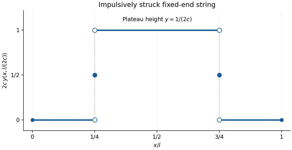
Fixed-end string at time l divided by 2c, showing the plateau and midpoint values at the two jump fronts
. Details. 
The product topology on consists of arbitrary unions of rectangles with , open. Such rectangles form a basis of a topology: every point lies in one, and intersections of two rectangles are rectangles with open factors.
If induce the factor topologies, setDefiniteness and symmetry are immediate. Each factor triangle inequality bounds its distance by the sum of the two relevant product distances; taking the maximum proves the product triangle inequality. A ball of radius is exactly , so every metric-open set is product-open. Conversely an open rectangle containing contains a product ball with radius the minimum of two suitable factor radii. Hence the maximum product metric induces precisely the product topology.
A compact space is one for which every open cover has a finite subcover. Let cover , with both factors compact; if either is empty the result is immediate. For each fixed and each , choose a rectangle containing and lying in a member of . The sets cover , so finitely many, indexed by , suffice. Their -neighbourhoods have open intersectioncontaining . The finitely many selected members of cover all of . Now the sets cover , so select finitely many of these by compactness of . Taking the union of their finite selections from gives a finite cover of the whole product. The product of two compact spaces is compact, without requiring the factors to be Hausdorff.
In the upper half-plane model, hyperbolic lines are vertical Euclidean rays and semicircles centred on the real axis, equivalently circle arcs meeting the real boundary orthogonally. A semicircle with endpoints is mapped to the imaginary axis byIts determinant is one, and its real endpoints map to . A vertical line is mapped to the imaginary axis by . Thus every hyperbolic line can be carried to a fixed one; composing one such map with the inverse of another proves transitivity of on the lines.
Reflection in is . Reflection in the unit semicircle is . The latter fixes the semicircle pointwise, is an involution, and preserves the hyperbolic metric because and . The vertical reflection similarly preserves . Their composition in the specified order is
Parallel hyperbolic lines have one common ideal endpoint and no interior intersection. Move the common endpoint to infinity by a Möbius transformation. The two lines are then distinct vertical lines . Their hyperbolic reflections have productwhose th power is . Since , no positive power is the identity.
Ultraparallel hyperbolic lines have no common endpoint or intersection. To see their common perpendicular explicitly, first map one line to the imaginary axis. The other has two boundary endpoints on the same side, say after possibly reflecting. It is a semicircle of centre and radius . The circle centred at zero with radius meets it orthogonally, since , and also meets the imaginary axis orthogonally. It supplies the common perpendicular. Map that perpendicular to the imaginary axis. Orthogonality then makes both lines semicircles centred at zero, of distinct radii . This normal form can also be obtained by a real Möbius transformation carrying the endpoints of the common perpendicular to . Their reflections are and , so their product isNo positive power of this dilation is the identity because and . Thus the product has infinite order in both nonintersecting cases. Geometrically the ultraparallel product is a translation along the common perpendicular through twice the separation of the lines.
If two hyperbolic lines intersect, move their intersection to the centre of the Poincaré disk model. Lines through the centre are diameters. Reflection in a diameter making Euclidean angle with the real axis is . The composition of two such reflections is the rotation . The Poincaré disk model is conformal, so the Euclidean angle difference is the hyperbolic intersection angle , up to sign and replacing it by , neither of which changes rationality of .
The rotation has finite order exactly when for some positive integer , equivalently . If in lowest terms, its order is . Conversely, the nonintersecting cases in part(a) have infinite order. Therefore
Use the original PDF constraints, whose right sides are and . Introduce nonnegative surplus variables , slack , and artificial variables :All seven variables are nonnegative. Phase I of the two-phase simplex method minimizes with initial basis . The initial simplex dictionary isEnter and leave : the ratio test gives . Substituting givesNow enter and leave . The bounds from are , so the ratio test selects . The new dictionary isThe associated basic solution has and , which is a global minimum because artificial variables are nonnegative. Delete their columns for Phase II. In the remaining basis the objective isFor , both reduced costs are nonnegative, so the simplex method has reached the optimum at :For , the coefficient of is negative. Enter ; the ratio test gives from and from , so leaves. Eliminating givesand henceThe two reduced costs are now positive, so is optimal andAt the whole feasible edge from to is optimal; both value formulas agree. These dictionaries explicitly carry out both phases rather than inferring the answer solely from a feasible-region sketch.
The monic orthogonal polynomial is orthogonal to every polynomial of degree less than , since form a basis of that polynomial space. Let be its distinct interior roots at which its sign changes, and put , with if . The real polynomial has constant sign throughout : multiplication by each linear factor removes its corresponding sign change, while even-multiplicity roots do not change sign. It is not identically zero. Since , its weighted integral is nonzero.
If , orthogonality instead gives , a contradiction. Thus . Degree also gives , so and all roots have multiplicity one, with no roots left outside the interval. Therefore there are exactly distinct simple zeros in . The weighted inner products are understood to exist, as required by the stipulated orthogonality.
Let , and set , . Expansion of the tridiagonal determinant along its last row givesFor the second term, the last-row entry is , its cofactor has negative sign, and the remaining minor has last-column entry multiplying ; their product is . Thus and have identical initial values and recurrence, and induction provesThe eigenvalues of the Jacobi matrix are precisely the roots of this characteristic polynomial. Part(a) therefore gives all eigenvalues simple and lying strictly in . This conclusion follows from orthogonality as well as symmetry; symmetry alone would establish real eigenvalues but not their interval location.
Work in the finite-dimensional vector space implicit in the requested matrix representation and . Put , with . These form an increasing sequence ending in , and . Choose a basis of , extend it to a basis of , and continue until a basis of is obtained. Each basis vector introduced at stage maps into the span of vectors chosen at earlier stages. Its matrix column can therefore have nonzero entries only in earlier rows. This proves that the matrix is strictly upper triangular.
For a strictly upper-triangular matrix , a nonzero contribution to requires an index chain . No such chain has links among indices. Consequently . An example with exact index four is the Nilpotent Jordan blockHere has entry one in position and all others zero, while .
In the adapted basis, is upper triangular with diagonal entries one, so all its eigenvalues are one. This does not persist for the product of two such matrices with unrelated adapted bases. TakeBoth square to zero, buthas characteristic polynomial and eigenvalues , neither equal to one. The obstruction is that the two nilpotent matrices need not admit a common triangularizing basis.
For inviscid flow that is also incompressible flow and irrotational flow with velocity potential , the Euler equations integrate to the Unsteady Bernoulli equationThe same applies throughout a connected irrotational fluid region; an additive time-dependent potential can absorb it. With gravity absent, fluid at rest at infinity and , it is .
Take the cylinder centre at laboratory position with , and define relative to this moving centre. The circulation-free potential flow satisfies Laplace's equation, decays at infinity, and has surface condition . The harmonic solution is consequentlyThe velocities are and , hence .
The time derivative must be taken at fixed laboratory coordinates, not fixed . At a fixed fluid point , , soSubstituting into the Unsteady Bernoulli equation gives the entire pressure fieldAt the cylinder surface this is . Pressure acts against the outward radial normal of the cylinder, so the force per unit length isAll steady terms cancel by trigonometric orthogonality. ThereforeThis identifies the added mass of a circular cylinder as the mass of displaced fluid per unit length. The solution assumes the ambient fluid is initially at rest and has no separately prescribed circulation; these select the usual pure translating-cylinder flow.
First write with . Direct multiplication givesThe inner product of its two columns isIf is orthogonal this is zero, and positivity of the bracket forces . The first column must then have length one, so . Thus , , and .
For the general QR decomposition, apply the Gram-Schmidt process to the ordered columns of the invertible real matrix . At stage , subtract projections onto the already chosen orthonormal vectors to get ; independence of the columns gives . Set . The matrix with columns is orthogonal, andis upper triangular. Its diagonal entry is strictly positive. This proves with the required properties.
Now suppose in dimension . Substitution of givesThe matrix is orthogonal, as are and , so this matrix and are orthogonal. Regard as upper triangular in blocks, with invertible diagonal blocks . The inverse is upper triangular in the same blocks, by solving the triangular block equations; multiplication by block diagonal preserves this pattern. Thus is block upper triangular.
An orthogonal block upper-triangular matrix is block diagonal. Indeed its first two columns are supported in the first two rows and are orthonormal, so span that first coordinate plane. Orthogonality of every subsequent column to them makes its first two entries zero. The remaining lower-right matrix is orthogonal; iterate this argument. Therefore with each orthogonal. The rule for diagonal blocks of products of block upper-triangular matrices givesEach is itself an upper-triangular real matrix with positive diagonal. The first calculation gives . Consequently , whence . Finally is a product of matrices commuting with , so . We have provedThis is positive-diagonal QR decomposition preserves a complex structure; the positivity convention is important in the two-dimensional step.
Expand the wavefunction in the complete orthonormal energy eigenstates. The Time-dependent Schrödinger equation makes each coefficient satisfy , soThe series is interpreted in the Hilbert space norm. Its norm is conserved because the phase factors have modulus one and the energy eigenstates are orthonormal. For initial data in the domain of the Hamiltonian operator, this is a strong solution of the equation; for any square-summable coefficients it gives the corresponding unitary time evolution.
In the two-dimensional span of the first two energy eigenstates, the measured observable has matrix . Its square is , and its trace is zero, giving eigenvalues . The orthogonal complement has eigenvalue zero. Thus the full spectrum is .
The normalized eigenstates for and are respectivelyThe lowest measurement outcome prepares up to an irrelevant overall phase. The subsequent unitary time evolution givesBy the Born rule, the probability of measuring the lowest eigenvalue again is the squared projection onto its one-dimensional eigenspace:This is the two-level quantum return probability with . At the probability is one; if the two energies happen to be equal it remains one for every time.
Articles by others on the same topic
There are currently no matching articles.