Past exam of the mathematics course of the University of Cambridge / 2016 / iii / Paper 207 (Biostatistics)

Use the usual clinical trial sampling assumption that all patients' responses are independent, with fixed positive arm sizes and positive known variances. Marginal normal distributions alone would not specify the variance of a treatment contrast without this assumption. Put ${\overline{Y}}_i=n_i^{-1}{\sum }_j{Y}_{ij}$, $v_i={\sigma }_i^2/n_i$, and $s_i=\sqrt{v_i+v_0}$. The sample mean contrast estimates ${\delta }_i$ and has standard error $s_i$. Thus the one-sided Wald statistics areLarge positive values of these Wald test statistics provide evidence against the respective null hypotheses.

The three independent sample means satisfy ${\overline{Y}}_i\sim \mathcal{N}({\mu }_i,v_i)$. A linear transformation of their joint multivariate normal distribution is again normal. The two treatment contrasts have covarianceWriting $m_i={\delta }_i/s_i$ and $\rho =v_0/(s_1{s}_2)$, their joint distribution isThe positive correlation coefficient arises from the shared control arm. Under positive variances, $0<\rho <1$.

Let ${\varphi }_{\rho }$ denote the centered unit-variance bivariate normal distribution density,The complement of rejecting either null hypothesis is $W_1\le c,W_2\le c$. Therefore the probability of at least one rejection isWhen both null hypotheses are true, this is the familywise error rate. If one null hypothesis is false, a rejection of that hypothesis is not a type I error, so the displayed probability is then an any-rejection probability rather than the familywise error rate.

Couple the Wald test statistics as $W_i=Z_i+{\delta }_i/s_i$, where the joint centered bivariate normal distribution of $(Z_1,Z_2)$ is fixed. Increasing either ${\delta }_i$ enlarges, pointwise in this coupling, the event $\{W_1>c\text{ or }{W}_2>c\}$. Its probability is consequently nondecreasing in each treatment effect.

If both null hypotheses hold, then ${\delta }_1,{\delta }_2\le 0$, so this probability is maximal at the joint boundary $(0,0)$. To check the familywise error rate across all configurations, suppose only hypothesis $i$ is true. A type I error then occurs only if $W_i>c$, with probability at most $1-\Phi (c)$, where $\Phi$ is the standard normal distribution function. This is no larger than the any-rejection probability at $(0,0)$, since that joint event contains $\{Z_i>c\}$. If neither null hypothesis is true, the familywise error rate is zero. Hence the least-favourable null configuration for type I error iswhere ${\Phi }_2$ is the centered bivariate normal distribution function with correlation coefficient $\rho$.

Choose a group sequential design. Randomize patients among the three arms, schedule interim analyses after prespecified amounts of information, and calculate the two Wald test statistics at each look. Prespecify efficacy boundaries and a futility rule; allow early stopping of an ineffective experimental arm or of the trial when sufficiently convincing efficacy evidence is obtained. Calibrate the boundaries for both repeated looks and the two shared-control comparisons so that the familywise error rate remains controlled. An alpha-spending function is one way to allocate the error probability across looks.

Two potential benefits are lower expected recruitment and shorter duration when a treatment is clearly effective or futile, and earlier identification of benefit or lack of benefit, reducing continued exposure to an ineffective experimental treatment. These benefits concern expected performance; the maximum sample size may still be required.

Two drawbacks are the extra operational work needed for rapid, reliable outcomes and confidential interim analyses, and more complicated inference: repeated testing requires adjusted boundaries, and ordinary fixed-sample effect estimates and confidence intervals can be misleading after data-dependent stopping. Continuing two comparisons against a shared control also requires care if an arm is stopped.

Use three states of a continuous-time Markov chain: disease-free $1$, pre-clinical $2$, and clinical $3$. The transition intensities are $\lambda =q_{12}>0$ for onset and $\nu =q_{23}>0$ for progression. Clinical disease is an absorbing state. The mandatory pre-clinical phase excludes a direct $1\to 3$ jump, and this untreated progression model has no reverse transitions.

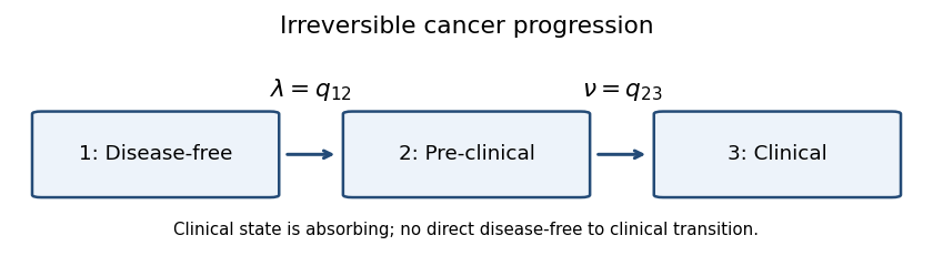
With row-vector probabilities and state order $(1,2,3)$, the generator matrix isIts rows sum to zero, so only the two off-diagonal transition intensities are unknown. This is a continuous-time multi-state model with sequential irreversible progression.

Starting in state $1$, the onset waiting time has the exponential distribution of rate $\lambda$. Thus the probability of onset before the next screen is $1-e^{-\lambda t}$. This counts individuals who have already progressed to clinical disease as well as those still pre-clinical.

Conditional on onset at time $u<t$, the Markov property makes the remaining progression time exponential with rate $\nu$. Thus the probability of clinical progression before the screen, conditional on that onset time, is $1-e^{-\nu (t-u)}$.

Integrating over the onset density gives the unconditional clinical probabilityThe probability of being pre-clinical at the next screen is insteadTogether with $P_{11}(t)=e^{-\lambda t}$ and the exponential distribution for a patient initially in state $2$, the transition matrix isThis equals the matrix exponential $e^{Qt}$. The assumed unequal intensities avoid a zero denominator; at $\lambda =\nu$ the continuous limit is $P_{12}(t)=\lambda t{e}^{-\lambda t}$.

Assume the 1000 individuals are initially disease-free. The event being counted is onset during the ten-year period, not occupancy of the pre-clinical state at its end. Using the estimated transition intensity as a constant onset rate and linearity of expectation, the expected number of onsets isThe first-order approximation $1000\times 0.005\times 10=50$ is close, but does not account for depletion of the disease-free group.

Let $A_i(s)$ be age in years at follow-up time $s$ and let $G_i\in \{0,1\}$ indicate the genetic risk factor. An age-dependent log-linear transition intensity model isHere $e^{{\theta }_0}$ is the onset baseline hazard for a 50-year-old without the factor; $e^{{\theta }_G}$ is the genetic hazard ratio, and $e^{{\theta }_A}$ is the hazard ratio per additional year of age. A smooth function of age could replace the linear age term if a constant age hazard ratio were unsuitable.

Under the stated constant multiplicative hazard ratios, the requested extrapolation is therefore the baseline rate times both multipliers:

Age changes during follow-up, so the generator matrix $Q(s)$ changes with time. The transition matrix must solve ${\partial }_{t_2}P(t_1,t_2)=P(t_1,t_2)Q(t_2)$, with $P(t_1,t_1)=I$. It is generally not the matrix exponential of one constant matrix; even $\exp (\int Q(s)ds)$ is not generally valid because the matrices at different times need not commute.

For example, write the age-dependent onset rate as $\lambda (s)$ and keep progression rate $\nu$ constant. ThenEven when the integrated onset rate is elementary, this remaining integral need not have an elementary closed form. Special cases can have closed forms; time dependence does not by itself prove universal impossibility.

For a tractable likelihood function, freeze age at its left-endpoint value, or a midpoint value, on each observation interval $[t_j,t_{j+1})$. The genetic covariate is already constant. This piecewise-constant covariate approximation gives a constant matrix $Q_j$ on each interval and a product of closed-form interval probabilities:Here $x_j$ is the observed state at $t_j$, and the likelihood function is conditional on the initial state. The approximation improves when intervals are short relative to the variation in the age effect.

Let $ϵ$ be the false positive rate for a genuinely cancer-free person, encompassing the harmless-tumour misclassification, and assume screening errors are conditionally independent given the latent states. A pre-clinical case tests positive with probability one; a clinical case is separately recognized. Thus a negative screen identifies latent state $1$, whereas a positive pre-clinical screen can arise from state $1$ or $2$. This is a Hidden Markov model with a screening misclassification model.

Conditional on the negative baseline screen, the state at year $0$ is $1$. The negative screen at year $2$ requires staying in state $1$ for two years and then testing negative. From that state, the positive screen at year $4$ can arise either with probability $ϵ$ while still disease-free or through pre-clinical disease. Consequently the conditional likelihood isIf the study instead specifies an initially disease-free patient and includes the baseline screening result in the likelihood function, its probability contributes a further factor $1-ϵ$, givingThe formulas use the positive emission for a pre-clinical screen, with no clinical diagnosis in this record. A persistent harmless-tumour subtype producing correlated screening errors would need an additional latent-state or emission specification; its likelihood is not determined by the single parameter $ϵ$.

In the SIR model, $S,I,R$ count susceptible, infectious, and recovered immune individuals. The closed population has $S+I+R=N+1$. Under homogeneous mixing, use the paper's mass-action infection convention: each susceptible has infection hazard function $\beta I$, so the population infection rate is $\beta SI$. Each infectious individual recovers with hazard function $\gamma$, giving population recovery rate $\gamma I$ and mean infectious duration $1/\gamma$.

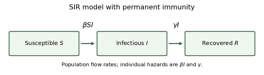
The arrows are one-way: recovered individuals are immune, and there are no demographic entries or exits. The transition intensities attached to the arrows are population flow rates, rather than individual hazard functions.

The deterministic SIR model follows the ordinary differential equationsUse $\beta \ge 0$ and $\gamma >0$. The state space is $S,I,R\ge 0$, $S+I+R=N+1$; summing the three equations proves conservation of this population. Infection is supported only where $S>0$ and $I>0$, and recovery only where $I>0$. The rates vanish at the corresponding boundaries, preventing negative compartment sizes.

This convention has an unnormalized population infection rate $\beta SI$, as required by the printed threshold. A convention with infection rate $\beta SI/(N+1)$ would use a differently scaled parameter.

Whenever $I>0$, divide the first SIR model equation by the recovery equation:The SIR susceptible-recovered identity follows by integrating from $R=0,S=N$, giving susceptibles as a function of recovered individuals:Population conservation then gives the infectious count:These identities extend continuously to the limiting state where the infectious count vanishes.

The infectious count in the SIR model obeys $\dot{I}=I(\beta S-\gamma )$. At the initial state, $\dot{I}(0)=\beta N-\gamma$, so initial epidemic growth requires the epidemic threshold for the closed SIR modelHere ${\mathcal{R}}_0$ is the basic reproduction number in this mass-action infection convention. Necessity also follows globally: $S(t)$ is nonincreasing, so if $\beta N\le \gamma$, then $\beta S(t)-\gamma \le 0$ for all time and $I(t)$ never increases. When $\beta =0$, growth is impossible.

At time zero the chain-binomial epidemic model has $B(0)\sim \mathrm{Bin}(N,\beta )$ and $C(0)\sim \mathrm{Bin}(1,1-e^{-\gamma })$, independently. The update gives $I(1)=1+B(0)-C(0)$. Since $B(0)\ge 0$ and $C(0)\le 1$, extinction at day one is equivalent to $B(0)=0$ and $C(0)=1$. Hence the one-day extinction probability isThis is the exact probability for the printed discrete-time approximation, which requires $\beta I(t)\delta t\in [0,1]$ wherever used. It should not be substituted for the distinct continuous-time extinction calculation.

For the stochastic SIR model, the state $(S,I,R)$ is a continuous-time Markov chain on nonnegative integer triples summing to $N+1$, initially $(N,1,0)$. Its only transitions areRates vanish when a proposed transition would leave the state space. Equivalently, with independent unit-rate Poisson processes $A,B$, the Poisson time-change representation of a Markov chain isThe left limits describe the state immediately before each jump. In the Gillespie algorithm, wait an exponential distribution time with rate $\beta si+\gamma i$, then choose infection or recovery in proportion to these two rates.

Initially, the infection and recovery transition intensities are $\beta N$ and $\gamma$. By competing exponential clocks, the first-event waiting time has distribution

The first event causes extinction precisely when it is recovery of the sole initially infectious individual. An infection would instead give two infectious individuals. The competing exponential clocks calculation therefore gives the first-event extinction probability

Write $a={\beta }^{\ast }=\beta N+\gamma$. If the first event is recovery, the epidemic has ended and a second event is impossible. If the first event is infection at time $s$, its density is $\beta N{e}^{-as}$, and the new state is $(N-1,2,0)$. The total next-event rate isThus, by the Markov property, the two-event probability in a stochastic SIR model by time one isEvaluate the first term as $\beta N(1-e^{-a})/a$. For the second, $b-a=a-2\beta$, soThereforeFor $N\ge 2$ and $\gamma >0$, the denominator ${\beta }^{\ast }-2\beta =\beta (N-2)+\gamma$ is positive. Event times are continuous, so inclusion or exclusion of the endpoint one makes no difference.

Throughout the survival questions, use the paper's notation $F(t)=\mathbb{P}(T>t)$ for the survivor function, not for a cumulative distribution function. To construct the Kaplan–Meier estimator, sort the distinct observed event times $a_j$. Let $r_j$ be the size of the risk set immediately before $a_j$, and $d_j$ the number of events at that time. The estimated conditional chance of surviving that event time is $1-d_j/r_j$. Multiplying these conditional probabilities givesA right censoring time reduces later risk sets but causes no jump itself. The usual interpretation as a population survivor function uses independent censoring.

The risk sets at the six event times are $(7,6,5,3,2,1)$, each with one event: the censoring between $t_3$ and $t_4$ removes the seventh individual before the fourth event. Thus the survivor estimate after the fifth event isConditional on reaching $t_4$, the event mass at $t_4$ is $1/3$, that at $t_5$ is $(2/3)(1/2)$, and that at $t_6$ is $(2/3)(1/2)(1)$. Hence the conditional event probabilities are

Now treat the seventh observation as an actual event at $t_4$, not as a censoring at that time. The risk sets are $(7,6,5,4,2,1)$ and the event counts are $(1,1,1,2,1,1)$. The Kaplan–Meier estimator therefore givesConditional on reaching $t_4$, the two events at that time have total probability $2/4=1/2$. Surviving them has probability $1/2$, which is then divided equally between the remaining two event times. Thus

For fractional event imputation, let $q_j$ be the fractional event weight assigned to the seventh individual at $t_j$. Its event contribution at $t_j$ is $q_j$. It belongs to the risk set at that time precisely for allocations at $t_j$ or later, so its fractional risk set contribution is ${\sum }_{j^{\prime }\ge j}{q}_{j^{\prime }}$. This justifies both parts of the hint.

For $(q_4,q_5,q_6)=(1/2,1/4,1/4)$, the fractional counts at the last three times areEarlier Kaplan–Meier estimator factors still give survival $4/7$ immediately before $t_4$. ConsequentlyThe three values are ${\hat{F}}_5^0=1/7\simeq 0.1429$, ${\hat{F}}_5^1=5/28\simeq 0.1786$, and ${\hat{F}}_5^{\ast }=4/21\simeq 0.1905$, in strictly increasing order. Spreading the censored individual's mass beyond $t_4$ raises the survivor estimate from the immediate-event imputation and moves it toward the original Kaplan–Meier estimator.

Assign the seventh individual's event weights $(1/3,1/3,1/3)$, the conditional probabilities obtained from the original Kaplan–Meier estimator. The last three fractional counts areTheir conditional event fractions are $1/3$, $1/2$, and $1$, exactly as in the original censored-data calculation. Hence the fractional allocation reproduces the original estimate:This illustrates self-consistency of Kaplan–Meier estimation: distributing the unobserved event according to the current conditional fitted event distribution leaves the fitted distribution unchanged. The first imputation in part (b) was not such a self-consistent allocation.

For a continuous proper event time with cumulative hazard function $H$ and survivor function $F(t)=e^{-H(t)}$, use the assumed inverse of $H$. For $u\ge 0$,Therefore the integrated-hazard transformation is unit exponential:This cumulative hazard probability transformation is the basis for the following survival-model residual diagnostics.

The transformed event time is unit exponential, and the transformed censoring time remains a censoring time because $H$ is increasing. Under independent censoring and a correctly fitted model, the Kaplan–Meier estimator of the survivor function for the Cox–Snell residuals $\hat{H}(x_i)$ should approximate $e^{-u}$.

Thus a logarithmic survivor plot should follow a straight line through the origin with slope minus one:The empirical plot is a step function around that line. Systematic curvature suggests model misspecification; the late part is less stable when the risk set is small. The retained event indicators $v_i$ must be used rather than treating censored residuals as complete event times.

Put $U=H(T)$ and $V=H(C)$, so $Y=\min (U,V)$ and $0\le \mathbb{E}Y\le \mathbb{E}U=1$. Its expectation is not generally one and depends on censoring. Under independent censoring, condition on $V=v$: the exponential distribution givesWriting $\Delta =1_{T\le C}$ for the observed event indicator, it follows that $\mathbb{E}Y=\mathbb{E}\Delta$. The exponential mean imputation under independent censoring therefore gives a modified Cox–Snell residual with known mean:On censoring, the added one is the expected remaining transformed lifetime, by memorylessness of the exponential distribution. This gives a mean-one variable, not necessarily another exponential variable. Equivalently, $M=\Delta -Y=1-Y^{\ast }$ is a martingale residual with mean zero. Independent censoring, or its appropriate conditional version, is essential for these identities; arbitrary informative censoring does not justify the correction.

Fit a model using the relevant covariates, calculate ${\hat{M}}_i=v_i-{\hat{H}}_i(x_i)$, and plot these martingale residuals against a candidate explanatory variable or against an included variable's value. A smooth systematic trend away from zero can indicate an omitted effect or an unsuitable functional form, such as a nonlinear age effect. After fitting an appropriate effect, the residual trend should diminish. The equivalent plot of ${\hat{Y}}_i^{\ast }$ has mean-one reference rather than zero.

For a nonnegative continuous event time $T$, the survivor function is $F(t)=\mathbb{P}(T>t)$, and its probability density function isThe hazard function is the instantaneous event rate conditional on being event-free at that time:If the event is certain to occur in finite time, the density is proper: ${\int }_0^{\infty }f(t)dt=1$, so $F(t)\to 0$. Since $F(0)=1$ and $F^{\prime }=-hF$, the cumulative hazard function is $H(t)=-\log F(t)$. Therefore a certain eventual event requires unbounded integrated hazard:If the lifetime has a finite upper endpoint, the same divergence occurs as that endpoint is approached, and $H$ is interpreted as infinite beyond it.

This is administrative censoring. Under the usual assumption that entry calendar time is independent of the subsequent event time, it is an example of independent censoring, not informative censoring: the planned study closure, rather than a patient's prognosis, determines the available follow-up. Uniform entry by itself does not prove that assumption; if entry date is associated with prognosis, independence must instead be justified conditionally on the relevant covariates. The calculations below use independence.

For administrative censoring with uniform entry, let entry time $A\sim \mathrm{Uniform}({\tau }_a,{\tau }_b)$. Then $C={\tau }_c-A$ has the uniform distribution on $[\ell ,r]$, where $\ell ={\tau }_c-{\tau }_b$, $r={\tau }_c-{\tau }_a$, and $d=r-\ell ={\tau }_b-{\tau }_a$. Its density and survivor function areDividing density by survival and integrating gives the censoring hazard and integrated hazard:The hazard function is undefined once no uncensored individuals remain. As $t\uparrow r$, it diverges like $1/(r-t)$ and the cumulative hazard function diverges logarithmically. This reflects the certainty of administrative censoring by the longest possible follow-up time, not dependence of censoring on the event process.

An individual has neither died nor been censored by time $t$ exactly when $T>t$ and $C>t$. Under independent censoring, this has probability $F_T(t)G(t)$. Thus the probability of leaving observation by either route isThe two pieces agree at $t={\tau }_c-{\tau }_b$. The expression counts the first of death and censoring, so it does not double-count individuals who would eventually experience both.

Choose an individual uniformly from the population. The law of total probability gives the population density and survivor function as mixtures:A hazard function is a ratio of density to survival, so averaging the densities does not average those ratios. Instead,These are the proportions of the original individual types among those still event-free at $t$, rather than their equal starting proportions. For example, a mixture of different exponential distributions progressively favours the lower-rate individuals. This population hazard of a survival mixture generally differs from $n^{-1}{\sum }_i{h}_i(t)$.

In the counting-process intensity in survival analysis, the counting process $N_i(t)$ jumps once if an observed event occurs; the at-risk process $Y_i(t)$ is one immediately before $t$ only while individual $i$ is still observed and event-free. Conditional on that information, the chance of an event in a short interval is $h_i(t)dt+o(dt)$ for an at-risk individual and zero otherwise. This is the meaning ofThe history ${\mathcal{H}}_{t-}$ is the filtration generated by the observed event and censoring histories, entry information, and available covariates strictly before $t$. In particular, it determines the current risk set but does not reveal future event times. The right-hand side is the infinitesimal compensator of a counting process; the equality is interpreted as an intensity statement to first order in $dt$.

Without censoring, $Y_i(t)=1_{T_i\ge t}$, so its unconditional expectation is survival:The distinction between $>$ and $\ge$ is immaterial for a continuous event time.

With independent censoring, the at-risk process is $Y_i(t)=1_{T_i\ge t,C_i\ge t}$. Independence and the common censoring survivor function $G$ give

Apply the tower property of conditional expectation to the intensity equation. Since $h_i(t)$ is a specified individual hazard function,As in the conditional equation, this describes the first-order expected increment of the observed counting process.

Let $N(t)={\sum }_i{N}_i(t)$ and $Y(t)={\sum }_i{Y}_i(t)$ be the total observed counting process and size of the risk set. When the individual cumulative hazard functions are all $H_0$, summing the conditional intensity equations givesReplace the expected increment by its observed value and divide by the predictable risk set size. Thus the Nelson–Aalen estimator in integral form iswith the integrand defined as zero when $Y(u)=0$. This is an integral against the step counting process, so each event time contributes its event count divided by the risk set just before that time. The Nelson–Aalen estimator estimates integrated hazard over times with observable risk; it does not supply information after observation has ended.

Use the allowed ratio-of-expectations approximation where $G(u)>0$. The unconditional numerator and denominator from part (b) giveThe common censoring survivor function cancels in this approximation. By differentiating the logarithm, its value is the population integrated hazard:This is not generally the arithmetic mean of the $H_i(t)$; it is the cumulative hazard function of the population mixture from part (a). The cancellation requires a common independent censoring law and adequate observation of the time range.

The approximation establishes approximate unbiasedness, not exact finite-sample unbiasedness. For a direct counterexample, take one uncensored individual with exponential distribution of rate $\lambda$. The Nelson–Aalen estimator is then $1_{T\le t}$, whose expectation is $1-e^{-\lambda t}$, whereas $\overline{H}(t)=\lambda t$. Thus it is not an unbiased estimator in general.

More explicitly, for independent individuals with a common event hazard $h$, the exact expected estimator isThis exhibits finite-sample bias of Nelson–Aalen estimation and dependence on $G$ when empty risk sets are possible. In a heterogeneous population, replacing the random ratios by ratios of their means introduces an additional approximation. On adequately observed intervals with large risk sets, the population-mixture expression is the appropriate large-sample target.