Past exam of the mathematics course of the University of Cambridge / 2017 / ib / Paper 2

For a linear map $\alpha :U\to V$ with $U$ a finite-dimensional vector space, the rank-nullity theorem isChoose a basis $u_1,\dots ,u_k$ of the kernel of a linear map and extend it to a basis $u_1,\dots ,u_k,v_1,\dots ,v_r$ of $U$. The vectors $\alpha (v_j)$ span the image of a linear map, because the kernel basis contributes zero. If ${\sum }_j{c}_j\alpha (v_j)=0$, then ${\sum }_j{c}_j{v}_j$ belongs to the kernel and is a combination of the $u_i$; independence of the extended basis makes every $c_j=0$. Thus the image basis has $r$ elements and $\dim U=k+r$, proving the theorem.

For a rank-two map on ${\mathbb{R}}^3$, the direct sum occurs for $\alpha (x,y,z)=(x,y,0)$: its kernel is $\mathbb{R}{e}_3$ and its image is $\mathrm{span}(e_1,e_2)$. It fails for $\beta (x,y,z)=(y,z,0)$: the kernel is $\mathbb{R}{e}_1$, contained in the two-dimensional image $\mathrm{span}(e_1,e_2)$. The rank-nullity theorem fixes the sum of the dimensions, but does not imply zero intersection.

A unique factorization domain is an integral domain in which every nonzero nonunit is a finite product of irreducible elements, uniquely up to reordering and multiplication of factors by a unit in a ring. A principal ideal domain is an integral domain in which every ideal is generated by one element.

Gauss lemma for polynomials says that over a unique factorization domain $D$, the product of two primitive polynomials is primitive, and the polynomial content satisfies $c(fg)=c(f)c(g)$ up to a unit. In particular a primitive polynomial of positive degree is irreducible over $D$ exactly when it is irreducible over the fraction field of $D$. Consequently a polynomial ring over a unique factorization domain is itself a unique factorization domain.

The Eisenstein criterion says that if $f(X)=a_n{X}^n+\cdots +a_0\in D[X]$ has $n\ge 1$ and there is a prime element $p$ with $p\nmid a_n$, $p\mid a_j$ for every $j<n$, and $p^2\nmid a_0$, then $f$ is irreducible over the fraction field. If $f$ is primitive, it is also irreducible in $D[X]$. Over $\mathbb{Z}$ one may take $p$ to be an ordinary prime number. The primitivity qualification prevents a nonunit constant content from being overlooked.

Take $\boxed{R=\mathbb{Q}[X]}$ and, for the next clause, its subring $S=\mathbb{Z}[X]$. Division with remainder makes $R$ a Euclidean domain, with the degree as Euclidean size for nonzero polynomials. For completeness, a nonzero ideal of $R$ contains a polynomial $g$ of least degree; division of any member by $g$ leaves a smaller-degree remainder in the ideal, so that remainder must vanish. The ideal is therefore $(g)$; the zero ideal is already principal. Thus $R$ is a principal ideal domain.

For the same pair, $\boxed{S=\mathbb{Z}[X]\subset \mathbb{Q}[X]}$. Since $\mathbb{Z}$ is a unique factorization domain, Gauss lemma for polynomials proves that $S$ is a unique factorization domain.

To prove that $S$ is not a principal ideal domain, consider the ideal $I=(2,X)$. A generator $g$ would divide 2 and $X$. Divisibility of 2 forces $g$ to be a nonzero constant integer; divisibility of $X$ then forces that integer to divide its coefficient 1, so $g=\pm 1$. This would make $I=S$. But evaluation at $X=0$ followed by reduction modulo 2 maps every element of $I$ to zero and maps 1 to one. Hence $1\notin I$, a contradiction. This is the integer polynomial ring is not a principal ideal domain example, with both clauses satisfied by a single inclusion.

The uniform convergence condition on a set $X$ isThe index $N$ is independent of $x$; this is stronger than pointwise convergence.

Fix $x_0\in \mathbb{R}$ and $ϵ>0$. Choose one $N$ such that $|f_N(x)-f(x)|<ϵ/3$ for every $x$. The continuity of $f_N$ at $x_0$ gives $\delta >0$ with $|f_N(x)-f_N(x_0)|<ϵ/3$ whenever $|x-x_0|<\delta$. The triangle inequality then givesSince $x_0$ was arbitrary, $\boxed{f\text{ is continuous on }\mathbb{R}}$, the uniform limit theorem. Continuity of each approximant need not be uniform continuity.

No: local uniform convergence need not be global uniform convergence. For a bounded counterexample use the continuous functions $f_n(x)=\min (1,|x|/n)$ and $f(x)=0$. On any fixed interval $[-M,M]$, for $n>M$,Thus there is locally uniform convergence to zero. On all of $\mathbb{R}$, however, ${\sup }_x|f_n(x)-f(x)|=1$ for every $n$, so uniform convergence fails. The cutoff needed to control the tails cannot be chosen independently of the interval.

The continuity condition at $x\in X$ between metric spaces isThe function is continuous when this holds at every $x$.

If $f$ is continuous and $U\subseteq Y$ is an open set, take $x\in f^{-1}(U)$. Some $ϵ$-ball around $f(x)$ lies in $U$. Continuity gives a $\delta$-ball around $x$ mapped into that ball and hence contained in $f^{-1}(U)$. Thus $f^{-1}(U)$ is open, including the empty set, in the notation for the image and preimage of a function.

Conversely, suppose every open set has open preimage. For fixed $x$ and $ϵ>0$, the preimage of the open ball $B_e(f(x),ϵ)$ is open and contains $x$, so contains some $B_d(x,\delta )$. This gives the displayed metric definition. Therefore $\boxed{f\text{ is continuous}⟺f^{-1}(U)\text{ is open for every open }U}$.

Let $X=\mathbb{R}$ with the usual metric and let $Y=\mathbb{R}$ with the discrete metric, and take $f(x)=x$. Every subset of $Y$ is an open set, so the image of every open subset of $X$ is open: $f$ is an open map.

It is not continuous at any point. For $ϵ=1/2$, every $\delta >0$ allows a distinct $y$ with $|y-x|<\delta$, but the distance between $f(y)$ and $f(x)$ in the discrete metric is 1. Equivalently, the preimage of the open singleton $\{x\}\subset Y$ is not open in $X$. Thus $\boxed{\text{an open map need not be continuous}}$ even between metric spaces.

Oddness gives zero cosine coefficients. Integration by parts gives the sine Fourier coefficientsThe Fourier series of the piecewise smooth periodic extension converges to its value at interior continuity points. Termwise integration from 0 to $x$ is valid: on the interval between these points, which stays inside $(-\pi ,\pi )$, the partial sums of $\sum (-1{)}^{n+1}\sin (nt)$ are uniformly bounded by the geometric-sum formula, since $|1+e^{it}|$ is bounded away from zero. The Dirichlet test therefore gives uniform convergence there. Integrating givesThe integrated series is absolutely and uniformly convergent. ConsequentlyIndependently, the constant Fourier coefficient is $a_0={\pi }^{-1}{\int }_{-\pi }^{\pi }{x}^{2}dx=2{\pi }^2/3$. Comparison yieldsThe original sine series is not uniformly convergent on the whole open interval; that stronger assertion is unnecessary for the justified integration.

In electrostatics, Gauss's law is ${\oint }_{\partial \Omega }\mathbf{E}\cdot \mathbf{n}dS=Q_{\mathrm{enclosed}}/{ϵ}_0$, or locally $\nabla \cdot \mathbf{E}={\rho }_e/{ϵ}_0$, where ${\rho }_e$ is charge density and ${ϵ}_0$ is vacuum permittivity. Spherical symmetry makes the electric field radial, and Gauss's law givesChoose the additive constant of the electrostatic potential by $\varphi (\infty )=0$. Using $\mathbf{E}=-\nabla \varphi$ and continuity of potential across each charged shell givesThe field jumps at the shell surfaces, so the displayed formulas are for the requested open regions. The potential difference of the spherical capacitor is $\Delta \varphi =Q(1/a-1/b)/(4\pi {ϵ}_0)$. Thus its capacitance and electrostatic energy areThe energy follows either by charging work ${\int }_0^{Q}q/Cdq$, or directly from $W=({ϵ}_0/2)\int |\mathbf{E}{|}^2{d}^{3}x=Q^2(1/a-1/b)/(8\pi {ϵ}_0)$.

For constant fluid density $\rho$, steady Euler equations for an inviscid fluid under a conservative force per unit mass $-\nabla \Phi$ read $(\mathbf{u}\cdot \nabla )\mathbf{u}=-\nabla p/\rho -\nabla \Phi$. Here $\mathbf{u}$ is velocity, $p$ pressure and $\Phi$ potential per unit mass. Dotting with $\mathbf{u}$ givesThis is the Bernoulli equation. The constants can differ between streamlines. If density varies, the same derivation for a barotropic fluid replaces $p/\rho$ by ${\int }^{p}d{p}^{\prime }/\rho (p^{\prime })$; constant density is the appropriate water approximation here.

For the draining cone, the radius at height $h$ is $h$ and the horizontal area is $\pi h^2$. Both the free surface and the jet are at atmospheric pressure; their gravitational potential difference is approximately $gh$. The speed of the descending surface is smaller than the jet speed by the area ratio ${ϵ}^2/h^2$, so it can be neglected when $h\gg ϵ$. The Bernoulli equation then gives Torricelli's law, $U\simeq \sqrt{2gh}$. Conservation of mass givesHence the leading drainage time of a conical tank isRemoving the tip places the aperture at height of order $ϵ$, and the quasi-steady calculation fails in the last layer of that depth. Integrating down only to $h=O(ϵ)$ changes the displayed leading time by relative order $(ϵ/h_0{)}^{5/2}$; replacing the actual head $h-ϵ$ by $h$ introduces a larger, but still vanishing, relative correction of order $ϵ/h_0$. The formula is the ideal inviscid estimate under the question's stated approximation, not an exact law for the final transient or a real contracted jet.

A $100\gamma \%$ confidence interval is a pair of statistics $L(X)\le U(X)$ whose random interval satisfiesAn exact confidence interval has equality throughout. The probability refers to repeated sampling at a fixed unknown parameter; the endpoints are random before observation. It is not a posterior probability assigned to the parameter after seeing the data. Here $0<\gamma <1$.

The sample mean $\overline{X}$ has normal distribution $N(\mu ,1/n)$ because the observations are independent with known variance 1. The pivotal quantity $Z=\sqrt{n}(\overline{X}-\mu )$ has the standard normal distribution. Consequentlyand inversion gives the confidence intervalReplacing 1.96 by the exact $0.975$ normal quantile gives exact 95% coverage; the printed numerical value gives the usual rounded interval. No variance estimation or Student distribution is needed.

Let $U_{(1)}=\min (U_1,U_2)$ and $U_{(2)}=\max (U_1,U_2)$ be the order statistics. For the symmetric uniform distribution, each observation is above or below $\theta$ with probability $1/2$, independently. ThusSo $\boxed{[U_{(1)},U_{(2)}]}$ is an exact 50% confidence interval.

The observed interval $[10,11.5]$ contains values impossible under the sampling model. Both observations must lie within one unit of the parameter, so the interval of all compatible values is $[U_{(2)}-1,U_{(1)}+1]=[10.5,11]$. It contains the true parameter almost surely. A support-restricted confidence interval for a uniform location parameter can therefore reportMore precisely, the procedure $[U_{(1)},U_{(2)}]\cap [U_{(2)}-1,U_{(1)}+1]$ retains exact 50% unconditional coverage, since the second interval contains $\theta$ almost surely. The intersection is a nonempty interval for every sample in the model and equals $[10.5,11]$ for these data. Reporting the full compatible interval alone is also valid and has coverage one. On this sample's large-spread event it lies wholly between the observations; this does not turn the unconditional 50% procedure into a generally 100% procedure.

For a vector equality constraint, take the Lagrangian function in constrained optimizationThe sign of the multiplier is a convention; equality multipliers are unrestricted. The Lagrange sufficiency theorem says that if $x^{\ast }\in X$ is feasible and, for some ${\lambda }^{\ast }$, globally minimizes $L(\cdot ,{\lambda }^{\ast })$ over $X$, then $x^{\ast }$ globally minimizes the constrained objective.

Indeed for any feasible $x$, $f(x)=L(x,{\lambda }^{\ast })\ge L(x^{\ast },{\lambda }^{\ast })=f(x^{\ast })$. Thus $\boxed{x^{\ast }\text{ is a global primal minimizer}}$. The theorem requires a global Lagrangian minimum, not merely a stationary point. It needs neither differentiability nor convexity when stated in this form; those hypotheses can be used separately to establish the required minimum.

For the same multiplier convention, the Lagrangian dual problem isFor every feasible $x$ and every $\lambda$, the equality constraint implies $q(\lambda )\le L(x,\lambda )=f(x)$. Taking first the infimum over feasible $x$ and then the supremum over $\lambda$ proves weak duality:The inequalities remain meaningful with the usual extended-value conventions, including $q(\lambda )=-\infty$ when the Lagrangian is unbounded below. Equality of optimum values, or their attainment, does not follow from weak duality. If the sufficient pair in part (a) exists, it attains equality, since $q({\lambda }^{\ast })=L(x^{\ast },{\lambda }^{\ast })=f(x^{\ast })$.

Put $A=\mathrm{im}\alpha$. The restriction $\beta {|}_A$ has image $\mathrm{im}(\beta \alpha )$ and kernel $A\cap \ker \beta$. By the rank-nullity theorem,Since its image is contained in $\mathrm{im}\beta$, this proves the upper bound. Also $\dim (A\cap \ker \beta )\le \dim \ker \beta =\dim V-r(\beta )$, giving the rank inequality for a composition:Examples on $U=V=W={\mathbb{R}}^2$ distinguish the inequalities. Taking $\alpha =\beta =I$ gives equality in both. Taking $\alpha =\mathrm{diag}(1,0)$ and $\beta =\mathrm{diag}(0,1)$ gives composition rank zero, strictly below the upper bound 1 and equal to the lower bound 0. Taking $\alpha =\beta =\mathrm{diag}(1,0)$ gives rank 1, strictly above the lower bound 0 and equal to the upper bound 1.

For the final nilpotent linear map, repeated application of the lower bound gives $r({\alpha }^k)\ge 2n-2k$. Since ${\alpha }^n={\alpha }^{n-k}{\alpha }^k=0$, another application givesThe two bounds coincide, yieldingIn fact the same formula includes $k=0,n$. For $n=1$ the requested index range is empty and the assumptions force $\alpha =0$.

For nilpotent elements $a,b$ of the commutative ring, choose positive integers $r,s$ with $a^r=b^s=0$. The binomial theorem giveseach term has either $j\ge r$ or $r+s-1-j\ge s$. Also $(-a{)}^r=0$, $0\in N$, and $(ta{)}^r=t^r{a}^r=0$ for every $t\in R$. Thus $N$ is an additive subgroup stable under multiplication by arbitrary ring elements:Commutativity is essential to the simple binomial argument; an arbitrary sum of nilpotent elements in a noncommutative ring need not be nilpotent.

Consider all ideals containing $I$ and disjoint from the nonempty multiplicative subset $S$. This collection is nonempty because it contains $I$. The ascending chain condition for the Noetherian ring gives a maximal member $P$: otherwise repeatedly choosing a strictly larger member would give an infinite strictly ascending chain of ideals. Since $S$ is nonempty and $P$ misses it, $P\ne R$.

Suppose $ab\in P$ but $a,b\notin P$. Maximality implies that $P+(a)$ and $P+(b)$ both meet $S$, so write $s=p+ra\in S$ and $t=q+ub\in S$ with $p,q\in P$. Thenwhile closure under products gives $st\in S$, a contradiction. HenceThis proves the prime ideal avoiding a multiplicative subset result without needing $1\in S$. The assumptions themselves rule out $0\in S$, since every ideal contains zero.

A nilpotent element belongs to every prime ideal: if $a^r=0\in P$, repeated primality forces $a\in P$. Therefore $N\subseteq {\bigcap }_{P}P$.

Conversely, if $a\notin N$, none of its positive powers is zero. The multiplicative subset $S=\{1,a,a^2,\dots \}$ is disjoint from $(0)$. Part (b) supplies a prime ideal disjoint from $S$, hence not containing $a$. Thus $a$ is outside the intersection, proving the nilradical as the intersection of prime ideals identity:In the zero ring there are no prime ideals; the empty intersection is interpreted as the whole ring, which is also its nilradical. For nonzero rings this argument proves existence of a prime ideal whenever a nonnilpotent element is available.

The unheaded preliminary requests are addressed before the first example. A norm is a function $p:V\to [0,\infty )$ satisfying $p(x)=0$ exactly for $x=0$, $p(ax)=|a|p(x)$, and $p(x+y)\le p(x)+p(y)$. Its induced metric is $d(x,y)=p(x-y)$. Translation $T_v$ preserves this distance, and scalar multiplication satisfies $d(ax,ay)=|a|d(x,y)$, so both are continuous; multiplication by zero is constant.

The open unit ball determines the norm uniquely through its Minkowski functional:because $x/t\in B$ is equivalent to $p(x)<t$. This also works for $x=0$.

Under the given radial and convexity hypotheses, set $p_B(0)=0$ and $p_B(v)=1/\lambda (v)$ for $v\ne 0$. The finite symmetric segment along each line gives positivity, absolute homogeneity and $v\in B⟺p_B(v)<1$. If $s>p_B(x)$ and $t>p_B(y)$, then $x/s,y/t\in B$, and the stated convexity condition yields $(x+y)/(s+t)\in B$. Hence $p_B(x+y)<s+t$; taking $s\downarrow p_B(x)$ and $t\downarrow p_B(y)$ proves the triangle inequality. Thus this is a norm determined by a convex radial unit ball. The case $V=\{0\}$ is immediate.

For the coordinate box, the Minkowski functional is the supremum norm:Indeed $x/t\in B$ exactly when $t>{\max }_i|x_i|$.

The interior of the diamond is $B=\{(x_1,x_2):|x_1|+|x_2|<1\}$. Its Minkowski functional, or the uniqueness argument already proved, gives the L1 norm:The final unheaded set $C$ cannot be an open unit ball of a norm, because every norm ball is convex by homogeneity and the triangle inequality. Both $p=(9/10,0)$ and $q=(0,9/10)$ lie in $C$: their squared-distance expression is $101/100>1$. Their midpoint has that expressionso $(p+q)/2\notin C$. Thus $\boxed{\text{no norm has }C\text{ as its open unit ball}}$. The strict inequalities in the definition are respected by this explicit counterexample.

The residue theorem states that a meromorphic function with finitely many poles inside a positively oriented simple closed contour and none on it satisfies ${\oint }_{C}F(z)dz=2\pi i\sum \mathrm{Res}(F;a)$. The function must be holomorphic on a neighbourhood of the contour and its interior away from those poles.

Write $J={\int }_0^{\infty }{x}^{1/2}\log x/(1+x^2)dx$ and $I={\int }_0^{\infty }{x}^{1/2}/(1+x^2)dx$. Both integrals converge absolutely. Use the principal complex logarithm in the upper half-plane, with $z^{1/2}=e^{\log z/2}$, and an upper semicircle of radius $R>1$ indented above zero by a clockwise semicircle of radius $ϵ<1$. The branch values on the negative real side are upper limits; equivalently use contours arbitrarily slightly above that side before taking a limit.

For $F(z)=z^{1/2}\log z/(1+z^2)$, the large arc is $O(R^{-1/2}\log R)$ and the small arc is $O({ϵ}^{3/2}|\log ϵ|)$, so both vanish. On $z=-x$ approached from above, $z^{1/2}=i\sqrt{x}$ and $\log z=\log x+i\pi$. The oriented negative segment therefore contributes $iJ-\pi I$, and the positive segment contributes $J$. The only enclosed pole is $i$, with residueConsequentlyComparing imaginary and real parts yields the upper-half-plane contour for square-root logarithmic integrals evaluation:

For unit $u$, put $A=I-2u{u}^T$. Then $A^T=A$ and $A^2=I$, so $A$ is an orthogonal matrix. The affine reflection in a hyperplane is $R(x)=Ax+2cu$. Hence $R(x)-R(y)=A(x-y)$ preserves the Euclidean norm and distance, and $R(x)=x$ whenever $u\cdot x=c$. Thus it is an Euclidean isometry fixing the hyperplane pointwise.

For $p\ne q$, any reflection exchanging them must have normal parallel to $p-q$, and its fixed hyperplane must contain their midpoint. These requirements determine the perpendicular bisector uniquely:Changing both signs of $u,c$ leaves the same reflection. It belongs to the orthogonal group $O(n)$ exactly when its translation term vanishes, that is, $c=0$. Since $c=(\Vert p{\Vert }^2-\Vert q{\Vert }^2)/(2\Vert p-q\Vert )$,To prove the finite reflection decomposition of a Euclidean isometry, first note that a distance-preserving map $g$ fixing zero preserves inner products by the polarization identity. Its values on an orthonormal basis $e_i$ form an orthonormal basis, and $g(x)\cdot g(e_i)=x_i$ shows $g(x)={\sum }_i{x}_{i}g(e_i)$. Thus $g$ is orthogonal.

Every orthogonal transformation is a product of at most $n$ linear reflections: if $g(e_1)\ne e_1$, reflect $g(e_1)$ to $e_1$ using the hyperplane normal $g(e_1)-e_1$, which passes through zero. The resulting orthogonal transformation fixes $e_1$, and its restriction to $e_1^{\perp }$ is handled inductively in dimension $n-1$. If $g(e_1)=e_1$, no initial reflection is necessary. Reflections on the complement extend by fixing $e_1$; the induction starts in dimension zero.

For an arbitrary isometry $f$, if $f(0)\ne 0$, first reflect $f(0)$ to zero across its perpendicular bisector with zero. Composing this one affine reflection with $f$ gives an orthogonal transformation. If $f(0)=0$, skip the initial reflection. ThereforeThe glide reflection $(x,y)\mapsto (x+1,-y)$ cannot use fewer than three: its determinant sign is negative, excluding zero or two reflections, while absence of fixed points excludes a single reflection. Three suffice by reflecting successively in $x=0$, $x=1/2$, and $y=0$.

The principle of stationary action, also called Hamilton's principle, requires $\delta {\int }_{t_1}^{t_2}Ldt=0$ for fixed-endpoint path variations. Here the original PDF has ${\dot{r}}^2$ in the radial kinetic energy; the TeX has lost that dot. With $m>0$ and $r>0$, the Lagrangian isThe Euler-Lagrange equation for each coordinate givesThe two conserved quantities are angular momentum $h=m{r}^2\dot{\varphi }$ and energy $E=\frac{m}{2}{\dot{r}}^2+\frac{m}{2}{r}^2{\dot{\varphi }}^2+km{r}^2$. By Noether's theorem, they arise respectively from rotational invariance and time-translation invariance of the action. The coordinate $\varphi$ is a cyclic coordinate, and $L$ has no explicit time dependence.

The conjugate momentum for each coordinate is $p_r=m\dot{r}$, $p_{\varphi }=m{r}^2\dot{\varphi }$. The Legendre transform $H=p_r\dot{r}+p_{\varphi }\dot{\varphi }-L$ gives the HamiltonianHamilton's equations areSetting $p_{\varphi }=h$ yields $m\ddot{r}=-V_{\mathrm{eff}}^{\prime }(r)$ with the effective potential $V_{\mathrm{eff}}=h^2/(2m{r}^2)+km{r}^2$.

For $k>0$ and $h\ne 0$, this potential tends to infinity both as $r\downarrow 0$ and as $r\to \infty$, and has its unique stationary point atThe effective potential stability criterion proves a stable circular orbit in a quadratic central potential, with $|\dot{\varphi }|=\sqrt{2k}$. For a small radial displacement $\eta$, $\ddot{\eta }+8k\eta =0$ to first order, so radial perturbations oscillate rather than grow. The diagram shows the centrifugal and quadratic contributions and their sum in dimensionless units:

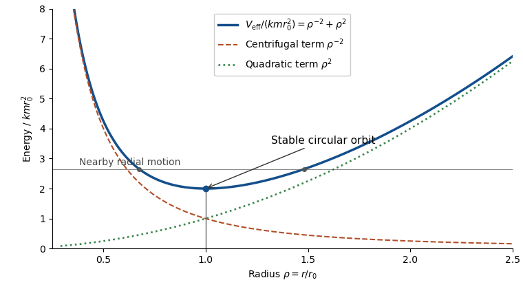
The printed paper only says that $k$ is constant. Its claimed positive-radius stable circular orbit needs the additional attractive-force assumption $k>0$ and nonzero angular momentum. For $k<0$ there is no such minimum; for $k=0,h\ne 0$ the effective potential is strictly decreasing. With $h=0,k>0$, the minimum is at the origin and is not a positive-radius circular orbit. These cases are not represented by the diagram.

Put $\varphi =R(r)\Theta (\theta )Z(z)$ in the Laplace equation in cylindrical coordinates. Separation of variables first gives ${\Theta }^{\prime \prime }+m^2\Theta =0$; $2\pi$-periodicity forces $m=0,1,2,\dots$, with angular factors $\cos m\theta ,\sin m\theta$ (only the constant for $m=0$). Taking $Z^{\prime \prime }={\kappa }^{2}Z$ givesFor $\kappa >0$ the separated modes are thereforeHere $J_m$ and $Y_m$ are the Bessel function of the first kind and the Bessel function of the second kind. For the opposite sign $Z^{\prime \prime }=-{\kappa }^{2}Z$, the modes instead involve $I_m(\kappa r),K_m(\kappa r)$, the modified Bessel functions, paired with $\cos \kappa z,\sin \kappa z$. At zero separation constant use $Z=C+Dz$ and $R=A{r}^m+B{r}^{-m}$ for $m\ge 1$, or $R=A+B\log r$ for $m=0$. Superpositions over the integer angular orders and appropriate sums or integrals over the separation parameter give the general separated expansion; boundary conditions select its spectrum and coefficients. Regularity at the axis excludes $Y_m,K_m,r^{-m},\log r$ terms.

For the specified decaying side data, bounded separated modes use $e^{-\kappa z}{J}_m(\kappa r)$. A particular solution isAll three denominators are nonzero. Each term satisfies the radial Bessel differential equation, is regular at the axis and bounded for $0\le r\le 1,z\ge 0$, and substitution at $r=1$ gives the stated side values. The modes behave as $r^m$ at the axis, so their apparent angular dependence there causes no singularity.

There is an actual nonuniqueness in the printed problem: no values are specified at $z=0$. If $j_{0,1}$ is the first positive zero of $J_0$, then for every real $a$,is another bounded solution with the same side values. It remains smooth at the axis and even decays as $z\to \infty$. This explicitly proves that side boundary data do not determine a bounded harmonic function in a half-cylinder. Thus the boxed expression supplies a bounded solution; the phrase “the bounded solution” is not justified without an additional base boundary condition. The PDF has $z\ge 0$, whereas the TeX transcription displays $z>0$.

For the quantum harmonic oscillator, the Time-independent Schrodinger equation iswith $m,\omega ,\hslash >0$. The given dimensionless coordinate yields ${\psi }_{\xi \xi }+(2E/(\hslash \omega )-{\xi }^2)\psi =0$. Substituting the Gaussian factor givesBy the supplied normalizability fact, $f$ is a nonzero polynomial. If its degree is $n$, comparison of the leading coefficient forces $2E/(\hslash \omega )-1=2n$. Conversely, at this value the coefficient recurrenceproduces a degree-$n$ polynomial with parity $n$: start with a nonzero constant for even $n$ or a nonzero linear coefficient for odd $n$, and the recurrence terminates at degree $n$. This is a multiple of the Hermite polynomial. Its product with the Gaussian is square integrable and can be normalized. Therefore all and only the allowed energies are