Past exam of the mathematics course of the University of Cambridge / 2019 / ia / Paper 2

The characteristic polynomial of the homogeneous linear ordinary differential equation isso its complementary solution is $A{e}^{3x}+B{e}^{-x}$. Because the forcing contains the resonant factor $e^{-x}$, set $y=e^{-x}v$. Substitution givesWriting $w=v^{\prime }$, a polynomial particular solution of $w^{\prime }-4w=-16x$ is $w=4x+1$, and hence $v=2x^2+x$. ThusBoundedness as $x\to \infty$ forces $A=0$, while the initial condition $y(0)=1$ gives $B=1$. Therefore

Substituting the proposed form $\mathbf{v}(t)=e^{\lambda t}\mathbf{u}$ into the linear system of ordinary differential equations givesIf $\lambda$ is not an eigenvalue of $B$, the matrix $\lambda I-B$ is invertible, soprovides the required particular solution.

In the stated two-dimensional case,and therefore $\mathbf{u}=(3,2{)}^T$. The eigenvalues of $B$ are $\pm \sqrt{3}$, with corresponding eigenvectors $(\sqrt{3},1{)}^T$ and $(-\sqrt{3},1{)}^T$. Adding the general solution of the homogeneous system yields

Since the natural logarithm is increasing, comparison with an integral givesThe lower bound is $n\log n-n+1$. Dividing all three expressions by $n\log n$ and applying the squeeze theorem gives

Stirling formula states

Every allocation is determined by the set of $n$ children on the red bus, so there are $\left(\genfrac{}{}{0ex}{}{2n}{n}\right)$ equally likely allocations. Exactly one places every boy on red and every girl on green. HenceApplying Stirling formula to the numerator and denominator gives the central binomial coefficient asymptoticand therefore

Independence of random variables and the two unit-rate exponential distributions giveThe linear transformationhas determinant $2$ and inverseThe inequalities $x,y\ge 0$ become $8v/3\le u\le 3v$. By the change-of-variables formula for probability densities,The variables $U$ and $V$ are not independent: the support of their joint density is a wedge rather than a Cartesian product of one-dimensional supports. For example, conditioning on a positive value of $V$ constrains $U$ to a finite interval depending on that value.

The Taylor expansions about $t_n$ areAdding them cancels the odd powers of $h$ and givesThus the centred finite difference has truncation error $O(h^2)$, so $\boxed{\alpha =2}$.

The characteristic equation of a linear recurrence isIts repeated root givesSince $t_n=nh$, this can be written $y_n=A+(B/h)t_n$, exactly the discrete form of the continuous solution $y(t)=C+Dt$ of $y^{\prime \prime }=0$.

The identityshows that $y_n^{(p)}=h^3{n}^3/6$ is a particular solution. Combining it with the homogeneous solution from part (b) givesThe condition $y_0=0$ gives $A=0$, and $y_{-1}=y_1$ gives $B=-h^3/6$. HenceThe exact initial-value solution is $y(t)=t^3/6$. Since $N=1/h$,Thus the absolute endpoint error is $h^2/6$, consistent with the second-order truncation error of the centred scheme.

Substitute the power series $y={\sum }_{n\ge 0}{a}_n{x}^n$ and compare the coefficient of $x^n$. This givesorThe two arbitrary coefficients $a_0,a_1$ determine all solutions. The condition $y^{\prime }(0)=0$ sets $a_1=0$, leaving the even series. It terminates precisely when ${\lambda }^2=(2k{)}^2$ for some nonnegative integer $k$. Therefore the permitted real values are $\lambda =0$ or $\lambda =\pm 2k$ for $k\ge 1$; these are the even Chebyshev polynomials up to normalization.

The degrees below six occur for $\lambda =0,\pm 2,\pm 4$. Taking $a_0=1$, the corresponding polynomials are

For the forced equation, try $y=a_0+a_2{x}^2+a_4{x}^4$. Comparing the coefficients of $x^4,x^2,1$ givesThus one polynomial satisfying $y^{\prime }(0)=0$ is

Put $\Delta =T_0-T_{\infty }$. Before either forcing term acts, Newton's law of cooling gives

Integrating the equation through $t=1$ gives the jump condition for an impulseFor $1<t<2$ the equation is again homogeneous, so propagation of the post-jump temperature givesTherefore

For $t>2$, the Heaviside step function contributes a constant unit forcing. Solving the resulting first-order linear differential equation from the value at $t=2$ gives

The cups have equal temperatures up to the intervention at $t=1$. For the later recrossing, subtract the formula for $T_2$ from that for $T_1$ and set the result to zero:Writing $z=e^{-a(t-2)}$ gives $z=(1+a{e}^{-a}{)}^{-1}$. Hence the nontrivial meeting time is

Using the Taylor expansionwe obtainWhen cooling is negligible, the milk lowers the temperature by one unit at $t=1$. The hot-water term begins at $t=2$ and raises it at one unit per unit time, so one further unit of time is needed to erase the deficit.

Along a trajectory, the chain rule givesThus $\boxed{H=x^2+y^2-y^4}$ is a first integral, and every trajectory lies on one of its level sets.

A critical point of a dynamical system satisfies $x=0$ and $y-2y^3=0$, so the critical points areThe Jacobian matrix of the vector field isAt the origin its eigenvalues are $\pm i$. Moreover, $H=x^2+y^2+O(y^4)$ has a strict local minimum there, so the origin is a stable center of a planar dynamical system. At either other critical point,has eigenvalues $\pm \sqrt{2}$, so both points are unstable saddle points. Their common value $H=1/4$ identifies the special separatrices shown below.

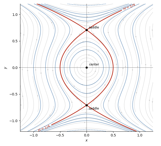
The initial point has $H=1/4$. On the branch leaving $(1/2,0)$ toward negative $y$,Since $\dot{y}=-x$, the required scalar equation isIts solution isAt $(x,y)=(1/4,-1/2)$, this requires $\tanh (t/\sqrt{2})=1/\sqrt{2}$. Using the inverse hyperbolic tangent,

The Kolmogorov axioms for a probability measure $\mathbb{P}$ are nonnegativity, normalization $\mathbb{P}(\Omega )=1$, and countable additivity on pairwise disjoint events. For $\mathbb{P}(B)>0$, conditional probability is defined byBecause the events $A\cap B_i$ are pairwise disjoint and their union is $A$, countable additivity gives the law of total probabilityFor any $j$ with $\mathbb{P}(A)>0$, the definition of conditional probability and this identity give Bayes theorem:

The prior probabilities of choosing the two urns are equal. Their white-ball probabilities areBy Bayes theorem,

The two possible ways to observe one ball of each colour have probabilitiesConditioning on their union therefore gives

Urn $i$ has $2^i$ balls, so a draw from it is white with probability $2^{-i}$. Given that the first ball is white, Bayes theorem gives the posterior probabilityAfter replacement, the second draw is conditionally independent of the first given the urn. HenceConsequently $\boxed{p(n)\to 1/3}$.

Let $h_k$ be the probability that the simple random walk started at $k$ hits $n$ before zero. The first-step analysis recurrence and boundary conditions areIf $p\ne q$, the characteristic equation of a linear recurrence has roots $1$ and $q/p$, so the boundary conditions giveIf $p=q=1/2$, the repeated root gives the limiting formula $\boxed{h_m=m/n}$. This is the gambler's ruin probability.

For a fixed integer stake $a\le N$, the fact that $a$ divides $N!$ lets us measure Patricia's wealth in units of £$a$. She starts at $M=N!/a$ and succeeds upon reaching $2M$. The formula above factors asFor $p=18/37$, $r=19/18>1$, so this probability increases as $M$ decreases. She should therefore choose the largest stake, $\boxed{a=N}$. For $p=19/37$, $r=18/19<1$, so the probability increases as $M$ increases; she should choose the smallest stake, $\boxed{a=1}$.

For every $u\in {\mathbb{R}}^2$,The right-hand side is a normal random variable by the definition of a bivariate normal distribution. Therefore every linear combination of the coordinates of $AX$ is normal, so $\boxed{AX\text{ is bivariate normal}}$.

For every $\lambda \in {\mathbb{R}}^2$, the scalar ${\lambda }^{T}X$ is normal with mean ${\lambda }^T\mu$ and variance ${\lambda }^{T}V\lambda$. The moment-generating function of a normal distribution therefore givesThus $\mu$ and $V$ determine the moment-generating function on all of ${\mathbb{R}}^2$. By the uniqueness theorem for moment-generating functions, they uniquely determine the probability distribution of $X$.

The covariance matrix isIf $\mathrm{Cov}(X_1,X_2)=0$, the moment-generating function in part (ii) factors into the product of the two marginal moment-generating functions. Thus $X_1$ and $X_2$ are independent random variables; this is the independence of uncorrelated jointly normal variables.

By bilinearity of covariance,ChooseThen $(X_1,Y)$ is bivariate normal by part (i) and has zero covariance, so $Y$ is a normal random variable independent of $X_1$. Hence $X_2=a{X}_1+Y$.

Let $D=R-L$ be right-arm length minus left-arm length. A linear combination of jointly normal random variables is normal, andwhileThus $D\sim N(2,3)$, and standardization of a normal random variable gives

Let $X_i=1_{A_i}$ be the indicator random variable of $A_i$. Then $X={\sum }_i{X}_i$, so linearity of expectation givesUsing variance of a sum andwe obtain

For the circular array, let $X_i$ indicate that bulbs $i$ and $i+1$ are both on, with indices read modulo $n$. Then $\mathbb{E}{X}_i=p^2$. Non-neighbouring indicators are independent, whileThere are $n$ individual terms and $2n$ ordered neighbouring pairs in the double covariance sum, so

The event $B$ is exactly $\{X\ge 1\}$. If $p=n^{-0.6}$, Markov inequality givesIf $p=n^{-0.4}$, then $B^c=\{X=0\}$ implies $|X-\mathbb{E}X|\ge \mathbb{E}X$. By Chebyshev inequality,Therefore $\boxed{\mathbb{P}(B)\to 1}$ in the second regime.