Past exam of the mathematics course of the University of Oxford / 2017 / Prelims / Mathematics V resit (A10142W1)

Source: released examination PDF, bundle pages 248–251.

Put $r=\sqrt{x^2+y^2}$. The definitions of the parabolic polar coordinates give $u^2=x+r$ and $v^2=-x+r$. Subtracting and multiplying these equations yieldsSince $u,v,y\ge 0$, taking the nonnegative square root givesThe Jacobian matrix has columns $(u,v)$ and $(-v,u)$. Its Jacobian determinant is thereforeHere the displayed fraction denotes the Jacobian determinant, as in the paper. The change of variables formula consequently gives $dxdy=(u^2+v^2)dudv$. The Jacobian determinant is positive except at the origin, and the definitions supply the unique nonnegative inverse throughout the region $y\ge 0$.

For $u=1$, the inverse parabolic polar coordinates give $y=v$ and $x=(1-v^2)/2$. For $v=1$, they give $y=u$ and $x=(u^2-1)/2$. Thus the requested curves are the upper halves of the parabolasThe first parabola has vertex $(1/2,0)$ and opens to the left; the second parabola has vertex $(-1/2,0)$ and opens to the right. Both pass through $(0,1)$ and are reflections of one another across the $y$-axis.

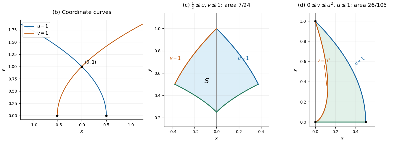
The inequalities become the rectangle $1/2\le u\le 1$, $1/2\le v\le 1$ in parabolic polar coordinates. The change of variables formula and the Jacobian determinant from a give the areaThe middle panel in b shows the curved region in Cartesian coordinates; its straight edges in parabolic polar coordinates explain the simple integration limits.

The first boundary is $u=1$. On $y=0$ in the first quadrant, the inverse parabolic polar coordinates give $v=0$. To identify the remaining curve, put $t=y^{1/3}\ge 0$. Its Cartesian coordinates satisfyHence $u=t$ and $v=t^2$, so this boundary is $v=u^2$. The condition $x\ge 0$ on this curve requires $0\le t\le 1$. Its endpoints are $(0,0)$ and $(0,1)$, while $u=1$ meets $v=0$ at $(1/2,0)$. These three arcs enclose exactlyEvery point in this region has $v\le u$, and therefore $x=(u^2-v^2)/2\ge 0$, as required. Using the Jacobian determinant, the area is

Let $V$ be a bounded region with piecewise smooth closed boundary $\partial V$, and let $\mathbf{F}$ be a continuously differentiable vector field on an open neighbourhood of its closure. The divergence theorem stateswhere $\mathbf{n}$ is the outward unit normal vector. Thus the volume integral of the divergence equals the outward boundary flux integral. For a region containing a hole, the outward unit normal vector on its inner boundary points into that hole.

For $r>0$, the chain rule gives $\partial r/\partial x_i=x_i/r$. Applying the product rule to the components of the vector field yieldsThe calculation is pointwise away from the origin; any extension of the vector field to the origin must be considered separately.

On the unit sphere, the outward unit normal vector is $\mathbf{n}=\mathbf{r}$ and $\mathbf{u}=\mathbf{r}$. Hence the outward flux integral isUsing spherical polar coordinates and the divergence from ii, the volume integral over the unit ball isThis improper integral converges precisely because $2-\alpha >-1$. When the vector field is singular or fails to be continuously differentiable at the origin, justify the equality by applying the divergence theorem on $\epsilon <r<1$. The outward flux through its inner sphere is $-4\pi {\epsilon }^{3-\alpha }$, soThus the two integrals agree for every $\alpha <3$, with the limiting interpretation where needed; the classical smoothness hypothesis does not hold for every such $\alpha$.

For $\alpha =3$, the divergence vanishes at every point with $r>0$, so its ordinary volume integral, ignoring the undefined single point, is zero. Nevertheless, the outward flux integral through the unit sphere is still $4\pi$:The hypotheses of the divergence theorem fail at the origin. Indeed $|\mathbf{u}|=r^{-2}$ there, so no continuous extension is possible. On the punctured region $\epsilon <r<1$, the divergence theorem remains valid: the outer flux is $4\pi$ and the inner flux is $-4\pi$. Unlike iii, this inner contribution does not tend to zero. The discrepancy therefore comes from the persistent flux at the singular point, rather than a failure of the divergence theorem under its hypotheses.

Write ${\partial }_i=\partial /\partial x_i$ and use $\times$ for the paper's wedge notation, which denotes the cross product. The given expression for the curl and the product rule giveApply the vector triple product identity $\mathbf{a}\times (\mathbf{b}\times \mathbf{c})=\mathbf{b}(\mathbf{a}\cdot \mathbf{c})-\mathbf{c}(\mathbf{a}\cdot \mathbf{b})$ separately to the two terms:Summing over the Cartesian basis vectors identifies the two directional derivatives and the two divergences:Here, for example, $((\mathbf{w}\cdot \nabla )\mathbf{v}{)}_j={\sum }_i{w}_i{\partial }_i{v}_j$. This proves the curl of a cross product directly from the formula supplied.

For the vector field $\mathbf{u}=(-y,x,0)$, the Cartesian formula for the curl gives

Apply the product rule inside the Cartesian expression for the curl:The first sum is the gradient of the scalar field and the second is the curl of the vector field. Thus the curl product rule for a scalar field is

Let $S$ be a piecewise smooth oriented surface with piecewise smooth boundary $\partial S$, and let $\mathbf{F}$ be a continuously differentiable vector field on a neighbourhood of $S$. The Stokes theorem statesThe boundary orientation is induced by the chosen unit normal vector $\mathbf{n}$ through the right-hand rule: with the right thumb along $\mathbf{n}$, the curled fingers indicate positive boundary traversal. Equivalently, when walking along the boundary with one's head pointing along $\mathbf{n}$, the surface lies to the left. An upward oriented disk therefore has counterclockwise boundary traversal when viewed from above. Reversing the orientation reverses both the line integral and the surface integral.

Choose the outward orientation on the upper half of the ellipsoid, giving counterclockwise boundary orientation on $C$ as viewed from $z>0$. Parametrize the boundary circle byThen $\mathbf{u}(\mathbf{c}(t))=(-\sin t,\cos t,0)={\mathbf{c}}^{\prime }(t)$, so the line integral isFor a direct surface integral, use the parametrized surfaceIts outward vector surface element is supplied by the cross productUsing the curl from a,The two integrals agree for every $\alpha >0$, verifying the Stokes theorem. Only the vertical component of the vector surface element enters, which explains the absence of $\alpha$ in the answer.

On the unit circle, the positively oriented unit tangent vector is $\mathbf{u}=(-y,x,0)$, and $|\mathbf{u}|=1$. Hence $d\mathbf{r}=\mathbf{u}ds$ andSince the scalar field $\psi$ has no $z$ dependence, the curl product rule for a scalar field givesOn the unit upper hemisphere $S_1$, the outward unit normal vector is $(x,y,z)$, so its vertical component is $z=\cos \theta$. Applying the Stokes theorem to the vector field $\psi \mathbf{u}$ therefore provesThe smoothness needed here is that $\psi$ extend as a continuously differentiable scalar field to a neighbourhood of the projected unit disk. The left side is a scalar line integral with respect to arc length; the positive boundary orientation is used when identifying it with the vector line integral.

For a nonzero integer $k$, direct integration giveswhereas ${\int }_{-\pi }^{\pi }1dx=2\pi$. The product-to-sum formulastherefore establish Fourier orthogonality: for positive integers $m,n$,Here ${\delta }_{mn}$ is the Kronecker delta. In particular the constant function is orthogonal to every nonconstant sine and cosine in this system. Integrating the given Fourier series, then multiplying it by $\cos (mx)$ or $\sin (mx)$ and integrating, isolates its Fourier coefficients. Using the permitted interchange of the sum and integral givesIf $f$ is an even function, then $f(x)\sin (nx)$ is an odd function, while $f(x)\cos (nx)$ is an even function. ThusThe Fourier series consequently reduces to a Fourier cosine series.

The function $x\sin (px)$ is an even function, so every Fourier sine coefficient is zero. Introduce the auxiliary integralFor a nonzero integer $k$, integration by parts givesConsequentlyFor $n\ge 1$, a product-to-sum formula yieldsIf $n\ne p$, this becomesThe exceptional Fourier coefficient at $n=p$ must be evaluated before dividing by $p-n$:Thus the full Fourier series isThis equality holds on $[-\pi ,\pi ]$ and by periodicity everywhere. Indeed the periodic extension is continuous at the joined endpoints, since both endpoint values are zero, and is piecewise smooth. The theorem on pointwise convergence of a piecewise smooth Fourier series therefore applies, including at the endpoints. The Fourier coefficients also decay as $n^{-2}$, making the resulting series absolutely and uniformly convergent.

Set $p=3$ and $x=0$ in the Fourier series from b. Since the function is continuous there, pointwise convergence of a piecewise smooth Fourier series givesIt follows thatThe $n=1$ and $n=2$ terms are $1/8$ and $-1/5$, respectively. Subtracting them gives the required absolutely convergent series:

Let the uniform string have constant tension $\tau >0$ and linear mass density $\mu >0$. Assume small transverse motion with $|u_x|\ll 1$, negligible longitudinal motion, and no external transverse force. If the string makes angle $\beta$ with the horizontal, then $\tan \beta =u_x$, and the small-angle approximation gives $\sin \beta \simeq u_x$ and $ds\simeq dx$ to first order.

The net upward force on the segment from $x$ to $x+\Delta x$ is thereforeBy Newton's second law, its mass $\mu \Delta x$ times its transverse acceleration equals this force, to the order retained in the small displacement model. Divide by $\Delta x$ and let $\Delta x\to 0$ to obtainThus the wave equation on a string iswhere $c$ is the wave speed. The horizontal force balance makes the horizontal component of tension constant; to first order it equals $\tau$.

The printed arguments $x-t$ and $x+t$ assume unit wave speed. For the stated wave equation with general $c>0$, the correct arguments are $x-ct$ and $x+ct$, as in the paper's subsequent formula. Equivalently, use rescaled time $\tilde{t}=ct$ to obtain the printed unit-speed form.

Introduce coordinates $\xi =x-ct$, $\eta =x+ct$ along the characteristic lines for the one-dimensional wave equation, and write $u(x,t)=U(\xi ,\eta )$. The chain rule givesso the wave equation becomesThus $U_{\xi }$ is independent of $\eta$, and integration gives the countertravelling decomposition of the one-dimensional wave equationConversely, differentiating this expression twice verifies the wave equation for any sufficiently differentiable $F,G$.

The two initial conditions giveDifferentiating the first and solving these two equations for the derivatives givesFor a fixed reference point $x_0$, their antiderivatives can be writtenSubstituting the two travelling arguments cancels the constants and combines the integrals. This proves D'Alembert's formula with initial velocity:At $t=0$ the integral vanishes, giving $u=f$; differentiating by the fundamental theorem of calculus gives $u_t=g$ there. These checks also fix the sign and the factor $1/(2c)$.

Here $f=0$ and $ct=1$, so D'Alembert's formula givesOnly the overlap $[1/2,1]$ with the support of the initial velocity contributes. ThereforeThe relevant interval is determined by the two characteristic lines for the one-dimensional wave equation through the observation point.

For a nonzero separable solution of the Laplace equation in polar coordinates, write $T(r,\theta )=R(r)\Theta (\theta )$ with $r>0$. Multiplying the partial differential equation by $r^2$ and dividing where $R\Theta \ne 0$ giveswhere $\lambda$ is a real separation constant. The resulting ordinary differential equations areThe equations continue across zeros of the factors by continuity. The radial equation is a Cauchy-Euler equation; putting $s=\log r$ changes it to $d^{2}R/d{s}^2-\lambda R=0$.

For positive separation constant, write $\lambda =k^2$ with $k>0$. The radial factors are powers, while the angular factors are sine and cosine:For zero separation constant, each transformed equation has zero second derivative, givingFor negative separation constant, write $\lambda =-k^2$ with $k>0$. The radial factors oscillate in $\log r$, and the angular factors are exponential functions:These exhaust the nonzero real separated solutions before imposing angular periodicity or regularity at the origin. The zero solution is also allowed. Since Laplace's equation is linear, sums of these separated solutions are solutions wherever the sums and required derivatives converge appropriately.

A temperature on the full unit disk must be single valued, so its angular factor and angular derivative are $2\pi$-periodic. For positive separation constant $\lambda =k^2$, this requires $k=n$ to be a positive integer. For $\lambda =0$, periodicity removes $D\theta$. For $\lambda <0$, no nonzero linear combination of $e^{k\theta }$ and $e^{-k\theta }$ is $2\pi$-periodic, so that case disappears.

The origin belongs to the disk, so a classical harmonic function must remain bounded and extend smoothly there. This excludes $r^{-n}$ and $\log r$. The remaining individual separated solutions are constants and $r^n(A_n\cos (n\theta )+B_n\sin (n\theta ))$. By superposition, the regular harmonic expansion on a disk isThe admissible Fourier coefficients are fixed by the boundary conditions. Smoothness at the origin can also be seen from $r^n\cos (n\theta )$ and $r^n\sin (n\theta )$ being the real and imaginary parts of $(x+iy{)}^n$, hence harmonic polynomials.

The constant function satisfies Laplace's equation and the prescribed Dirichlet boundary condition. In the harmonic expansion on a disk, its only nonzero coefficient is $A_0=1$. By the allowed uniqueness for the Dirichlet problem,

The boundary data consist of the third angular Fourier mode. Its regular radial factor in the harmonic expansion on a disk is $r^3$, soFor a direct check of Laplace's equation,Also $T(1,\theta )=\sin (3\theta )$. At the origin the apparent coordinate singularity is harmless: this is the harmonic polynomial $3x^{2}y-y^3$. The allowed uniqueness for the Dirichlet problem completes the identification.

The trigonometric identityshows that only angular Fourier modes $1$ and $3$ are required. Differentiating the harmonic expansion on a disk at $r=1$ multiplies the coefficient of each nonconstant Fourier mode by $n$. Thus $B_1=3/4$ and $3B_3=-1/4$, givingEach term is a regular harmonic function, and the radial derivative isThe Neumann compatibility condition for Laplace's equation holds becauseas is necessary by the divergence theorem applied to the gradient of a harmonic function.

The additive constant is undetermined. This Neumann boundary condition is unchanged by $T\mapsto T+C$, so the paper's blanket uniqueness assertion requires a normalization in this case. The uniqueness of the Neumann problem gives uniqueness up to a constant; prescribing $T(0)=0$, or zero mean temperature, selects the displayed answer with $C=0$.