Multiply the differential equation by . Sincethe Sturm-Liouville form isThe weighted inner product is consequently . These endpoints are singular: vanishes and diverges, though is integrable. The required boundedness of makes the boundary factors vanish, which is the fact needed in the integration identities below.
Use the real eigenfunctions, or insert a complex conjugate on the first factor for complex functions. Multiply by , do the same with interchanged, and subtract. Integration by parts givesThe boundary term vanishes because both functions and derivatives are bounded while . For distinct squared indices, orthogonality of Sturm-Liouville eigenfunctions therefore yieldsA second integration by parts, using the equation for , givesThus derivative orthogonality when the Sturm-Liouville potential vanishes givesThe index qualification matters. The source initially allows integer indices, so alone does not imply distinct eigenvalues: gives the same . Taking the conventional nonnegative labels makes the stated conclusion valid. For the polynomial solutions below, , so opposite indices are an explicit counterexample to an unqualified orthogonality claim.
For nonnegative integer , De Moivre's theorem makes its polynomial nature explicit:Every term is a polynomial of degree at most . For , the coefficient of is , so its polynomial degree is exactly . These are the Chebyshev polynomials . Their polynomial form also proves the required boundedness of the function and derivative at both endpoints. Negative labels reproduce and have degree .
The first three areUnder , their cross inner products become integrals of , and on . The constant-cosine integrals vanish, and also integrates to zero. Thus all three pairs are orthogonal. Their squared weighted norms are , respectively; more generally
For separation of variables, write . The exterior Laplace equation separates intoWith , angular regularity at the poles selects and the Legendre polynomial . The radial equation is , an Euler-Cauchy equation with solutions . Decay at infinity excludes the first branch for every , including its constant case. ThereforeThe expansion uses axisymmetric spherical harmonics. The written scalar boundary-value problem permits the term; any additional physical exclusion of that sector must be stated separately.
Separate the interior Helmholtz equation in the same angular basis. Each radial coefficient satisfiesFor , set . The equation becomes . Its regular solution is a Spherical Bessel function , up to a multiplicative constant. The second independent solution is singular as at the origin and is excluded. HenceOne may denote by as in the source. Its leading behaviour ensures regularity. Primes on below refer to its dimensionless argument; differentiating with respect to introduces the factor .
Put . Orthogonality of the Legendre polynomials lets us match each degree separately. Continuity of the field and its radial derivative givesEliminate by multiplying the first equation by and adding it to the second. A nonzero mode therefore requiresThis argument avoids dividing by a potentially zero boundary value. Apply the supplied recurrence with :Consequently spherical Helmholtz matching to a decaying harmonic exterior giveswhere for the sector.
The original PDF has an index error here: it prints rather than in the resulting eigenvalue condition. This cannot be repaired by silently choosing another normalization. If itself were zero at a positive matching root, the boundary equation would also give , contradicting uniqueness for this nonzero solution of a regular differential equation at that point.
A positive matching root gives . Substituting the root value requested by the question gives the intended expressionAfter the index correction in part (iii), this is indeed the lowest mode in the sector, because its condition is and its first positive root is . It is also the minimum over .
However, the literal scalar problem includes , for which matching gives . Its first positive root is , so the actual minimum for the written scalar equations and stated boundary conditions isAn explicit counterexample to the larger proposed minimum is , , with no angular dependence. At , both values are and both radial derivatives are .
To verify minimality, put . The radial problem is , , . Its Rayleigh quotient isFor this is the Dirichlet-Neumann interval problem, whose lowest eigenvalue is . The additional nonnegative terms increase with , proving the scalar minimum and the minimum-at- statement for the restricted family. A monopole-free magnetic multipole interpretation would exclude and yield the intended value, but that extra restriction is not supplied by the stated scalar model. The claim about the first zero is not valid for every as printed.
Write . Away from the source, the radial Laplacian gives . Through a small source-centred sphere, the outward flux of its gradient isThis identifies a unit Dirac delta at the source. More explicitly, for a smooth compactly supported test function , apply Green's second identity outside the radius- ball. The inner outward normal of that punctured domain is . The term has integral , while tends to . Thus , proving the distributional identityWhenever the integral converges, convolution with this Green function of the Laplacian solves the Poisson equation for Newtonian gravity:The harmonic term represents the homogeneous freedom and is fixed by boundary conditions. For an isolated finite mass distribution, regularity away from the prescribed sources and the normalization at infinity select .
Choose the polar axis in the source integration along the evaluation vector . The Euclidean distance then satisfies , givingFor the uniform ball, integrate its Newtonian gravitational potential in these spherical coordinates. With ,For , the inner integral isobtained from the antiderivative . ThereforeFor , split the radial integral at . Its two pieces are and . The Newtonian gravitational potential of a uniform solid sphere is consequentlyThe centre value follows by continuity, removing the intermediate . For , the same integral gives , so both the potential and first derivative match at the surface. Finally inside, while is directed inward and vanishes at the centre, checking the sign and normalization.
The only possible singularity of inside the contour is at , with residue . It is at most a simple pole; when , it is removable. Thus the residue theorem gives the Cauchy integral formula,for a counterclockwise simple contour containing once, with analytic on a neighbourhood of the contour and its interior. More generally the answer is , where the winding number accounts for multiple turns or reversed orientation. A clockwise simple contour has the opposite sign.
The integrand has simple poles at and . Only the first is inside the upper contour, and its residue isThe residue theorem therefore gives, for every ,On the upper semicircle, and . The estimation lemma bounds the arc contribution by . Hence the real-axis integral has the same limit, and taking its real part givesThe imaginary part vanishes independently because is odd. The real integral converges absolutely, since the denominator grows quadratically.
For , use . The interval traverses once counterclockwise, , and . ThusPut . The two simple poles areTheir moduli are and , so exactly is enclosed, for either sign of . Its residue isThe residue theorem yieldsThis also follows from the reciprocal affine sine integral after an angular shift. At , the original integral is directly , agreeing with the boxed formula. The displayed two-pole formulas require : at zero the contour integrand reduces to with a single pole. Thus the source's claim of two simple poles has this removable special-case exception.
The triangular function is real and even, so its Fourier transform reduces to a cosine integral:For , one integration by parts gives . Therefore the Fourier transform of a triangular function isThe zero-frequency value is the removable limit and also the area of the triangle. The transform is a squared sinc function, which explains its nonnegativity despite the oscillating Fourier exponential.
Under regularity and integrability conditions permitting the limits to pass through the integral, apply the difference quotient directly in time:For the spatial derivative, translate the integration variable in the first term:ConsequentlyThe second calculation is the Translation property of the Fourier transform applied to a difference quotient. These are the Fourier transform of a derivative identities. The stated decay removes boundary terms in the alternative integration-by-parts derivation; rigorous interchange of limits also requires suitable control, for example integrable derivatives. The formulas extend to tempered distributions.
Apply the identities from part (ii) twice. The second time derivative becomes and the second spatial derivative becomes . The Fourier transform method for the wave equation therefore givesFor each fixed wavenumber , this is a harmonic oscillator equation with angular frequency . At its solutions are affine in time rather than two independent oscillatory exponentials.
Zero initial velocity selects the cosine solution of the transformed equation:with the removable value one at . Since , the Fourier shift theorem giveswhere . This is triangular pulse splitting under the wave equation, a special case of the D'Alembert formula.
The two half-height triangles move in opposite directions at speed . Their sum initially reproduces the full triangle; once their supports are disjoint. The field vanishes outside , consistent with finite propagation speed. For it simply remains .
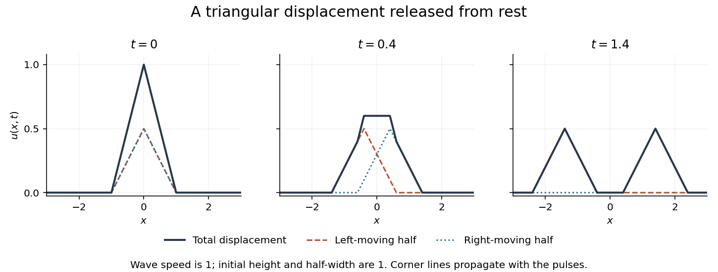
A triangular displacement released from rest splits into two translating half-amplitude pulses; their overlap adds
. Details. 
Because the triangular profile has slope discontinuities, this is a weak solution rather than a globally twice differentiable solution. The initial velocity is zero in the distributional or square-integrable sense, and pointwise away from the initial corners. A classical pointwise time derivative need not exist at those corners; for example near . The initial conditions must be interpreted consistently with this nonsmooth displacement.
For a constant orthogonal Cartesian coordinate change , the tensor component transformation law givesRepeated indices are summed. Each index of an ordinary Cartesian tensor contributes one factor of . A pseudotensor would have an additional determinant factor under an orientation-reversing transformation; the rules here concern ordinary tensors.
Define the outer product . Transforming each vector givesThus is a rank-two tensor, since it obeys the two-index tensor component transformation law. This is the component form of the tensor product of two vectors; its two indices are independent, not contracted.
Adding and subtracting the transpose uniquely separates a Cartesian second-rank tensor into its symmetric tensor and antisymmetric tensor parts:Then , and . Both parts transform as tensors because transposition commutes with the orthogonal similarity . Uniqueness follows by taking the symmetric and antisymmetric parts of any such decomposition.
The tensor contraction of a symmetric tensor with an antisymmetric one vanishes. Rename the two summed indices and use their opposite exchange symmetries:Hence . Using the decomposition from part (iii) givesThis is orthogonality of the real symmetric and antisymmetric matrix subspaces under the Frobenius inner product. It is a summed scalar identity, not an assertion about the unsummed products of individual entries.
Let be the rank-two tensor and the vector. The components of their tensor product are . Applying the transformation rules givesThe product therefore obeys the three-index tensor component transformation law, proving that is a rank-three tensor. Tensor-product order adds because no pair of indices is summed out.
Start from the three-index transformation law and contract the first two Cartesian indices:Orthogonality supplies , where is the Kronecker delta. The remaining factor is exactly the vector transformation rule. Therefore is a vector.
This tensor contraction removes two indices by pairing them through the Euclidean metric. In general nonorthonormal coordinates, contraction must use the appropriate metric or pair a covariant and a contravariant index; the bare repeated-lower-index sum relies on Cartesian orthonormal coordinates.
Write the curl and cross product with the Levi-Civita symbol, then use its contraction identity:Expanding with the product rule givesRecognize the divergence in the first and third terms, and the directional derivatives in the other two. The curl of a cross product identity is thereforeThe derivatives act on both vector fields. No assumption of vanishing divergence or spatially constant fields has been made.
Take both displacement coordinates positive to the right. The kinetic energy and elastic potential energy areThus the equations of motion are and . With , the generalized eigenvalue problem for small oscillations isIts determinant gives . Put . The two-mass three-spring normal modes haveBoth squared frequencies are positive because . Also , so and : the lower mode moves the masses in phase, and the higher mode moves them oppositely. A general mode is an arbitrary sinusoidal amplitude multiplying its fixed shape.
For equal masses these reduce to , and , . For unequal masses the vectors need not be Euclidean-orthogonal; they are orthogonal in the mass inner product, .
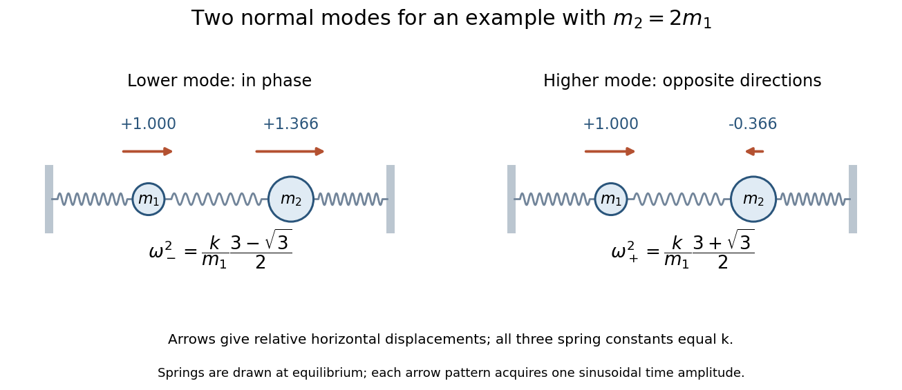
In-phase and out-of-phase mode directions for an illustrative unequal-mass system; arrow lengths show relative displacements
. Details. 
The displacement directions specified at release give . Let . By initial-data decomposition into two normal modes, write . Solving the two coordinate equations givesZero initial velocities remove the sine terms, soIn components,Substitution at zero gives , , and both derivatives vanish. For unequal masses both normal modes are generally present. When , , , so only the higher mode survives: and .
Since both initial displacements vanish, only sine terms are needed. Resolve the velocity into the two normal modes:Each modal initial velocity must be divided by its angular frequency to obtain its displacement amplitude. ThereforeExplicitly,At zero, both displacements vanish and differentiation gives . The motion combines the in-phase and out-of-phase modes, with opposite signed modal velocity coefficients. Their different frequencies produce changing constructive and destructive interference in the physical coordinates, so motion is transferred through the coupling spring. This does not require assuming equal masses or exact periodic transfer of all the energy.
Interpret the functions as maps on , so every reciprocal is defined. Let , , and . With the left factor applied last, direct function composition gives the Cayley tableThe table proves closure and identifies as the identity. Every element is its own inverse. Associativity is inherited from composition of maps, so the set is a group. The three nonidentity elements are commuting involutions.
Its subgroups areThere are no others: a subgroup containing two distinct nonidentity elements also contains their product, the third, and hence is the whole group; a subgroup containing just one has order two.
The abstract dihedral group has commuting generators with , for example a rectangle's half-turn and reflection in one axis. The assignment , , , respects products and is bijective. ThusThis is the group generated by sign reversal and reciprocation, a realization of the Klein four-group. The nonzero domain is essential; treating these as functions defined at zero would not give the stated group.
For a subgroup of a finite group , Lagrange's theorem statesThe left cosets partition the group and each has members, proving the formula. If is prime, the only divisors are one and , so or . Hence a group of prime order has no nontrivial proper subgroups.
The word “nontrivial” is necessary: is a proper subgroup of every prime-order group. Thus the source's shorter wording cannot literally exclude all proper subgroups.
The order of a group element is the least positive integer such that , or infinity if there is no such integer. In a finite group such a exists, because two powers among must coincide.
The powers are distinct: a repetition with exponents differing by less than would contradict its minimality. Division of any exponent by shows that these are all the elements of the cyclic subgroup . Thus . Applying Lagrange's theorem givesIn particular the identity has order one, and every nonidentity element has order greater than one. The divisibility assertion here concerns finite group order.
Let be prime and choose . Its order divides by part (iii), and cannot be one. Hence its order is , so its generated subgroup has the same number of elements as the whole group:This proves that a group of prime order is cyclic. In fact every nonidentity element is a generator. No commutativity assumption was needed; it follows from cyclicity.
For the intended finite nontrivial case, let have composite order . Choose a prime divisor of , with . Thenis a nontrivial proper cyclic subgroup of order . Indeed , and no smaller positive power is the identity because has order . Thus .
If the source also allows an infinite cyclic group, is a proper cyclic subgroup: its powers have even exponents and do not include . The trivial group, of order one, is an exception to the literal formulation “not of prime order”: it has no proper subgroup at all. The nontriviality assumption is therefore necessary for that general wording. These facts are instances of subgroups and quotients of a cyclic group.
A subgroup is a normal subgroup when conjugation by every group element preserves it:Equivalently, for every ; normality permits the cosets to inherit a quotient-group multiplication.
A group homomorphism is a map preserving multiplication:It consequently sends identity to identity and inverses to inverses, since and .
The image of a group homomorphism contains . If and lie in the image, then also lies there. The subgroup test proves .
The kernel of a group homomorphism is . It is nonempty and closed under for , so it is a subgroup. For any and ,Thus . Replacing by gives the reverse inclusion, provingFinally, if and , then . Thus forces , establishing injectivity. Conversely an injective homomorphism has trivial kernel, soNone of these arguments requires either group to be finite.
Label the triangle vertices counterclockwise. Let rotate by counterclockwise and let reflect across the line through vertex 1 and the midpoint of the opposite side. The dihedral group has elements , with and .
The action on vertices identifies them with these permutations, with the rightmost operation applied first:The minimal number of generators is two, and is one minimal generating set. They produce every displayed element. A one-element generating set would make the group cyclic, but every nonidentity element has order two or three, never six.
The vertex-action map preserves composition, hence is a group homomorphism from to the symmetric group . The displayed actions are all six distinct permutations of three vertices, so the map is both injective and surjective. ThereforeThis identification uses the convention , with the subscript counting polygon vertices.
For a group representation , a faithful representation is injective, equivalently only for . Thus no distinct group elements are represented by the same linear map.
Two equivalent representations are related by one fixed invertible change of basis: for every . The same must work simultaneously for all group elements.
An irreducible representation acts on a nonzero vector space and has no invariant subspace other than and the whole space. An invariant subspace is one carried into itself by every representing matrix.
The character of a representation isThe cyclic property of the trace makes it invariant under equivalence and constant on conjugacy classes. Its value at the identity is the dimension of the representation.
Denote the four listed matrices, in order, by . As permutation matrices, act on the four basis vectors by , and , respectively. Direct multiplication givesThese relations prove closure and show that each element is its own inverse. The identity is included and matrix multiplication is associative, so the matrices form a group.
The relations coincide with those of the Klein four-group : take its half-turn generator to , a reflection generator to , and their product to . All four matrices are distinct, so this assignment is a faithful representation of . It is the four-point regular representation of the Klein four-group.
Every matrix fixes , since it permutes its coordinates. Thereforeis a one-dimensional invariant subspace, nonzero and strictly smaller than the four-dimensional space. This proves the representation is reducible. In fact the four mutually orthogonal sign vectors , , and give invariant lines and completely diagonalize the representation, as in the normalized Hadamard matrix construction.
Write the finite cyclic group as , the source's . It is Abelian, so and every conjugacy class is a singleton: there are such classes.
Over the complex numbers, all its irreducible representations are one-dimensional. One direct proof is that the matrix representing has an eigenvector over ; its line is preserved by every power of that matrix and hence by the whole group. Irreducibility forces the line to be the whole representation space. Its eigenvalue must be an th root of unity.
The complex irreducible representations of a finite cyclic group are thereforeTheir generator values are distinct, so no two are equivalent. There are of them, and squared dimensions equal one, exhausting the sum of squares of irreducible representation dimensions: . Thus the list is complete.
For , let , so and . The character table isThe complex-field convention is essential. The preceding part used real matrices, but that does not make the one-dimensional classification valid over : conjugate nonreal characters combine into the two-dimensional irreducible real representations of a finite cyclic group. The character table and dimension-sum result used here have their usual complex meaning.
Articles by others on the same topic
There are currently no matching articles.