Source: Oxford's released examination PDF, pages 172–175, dated 19 June 2023; questions 1, 2 and 3 occupy pages 173, 174 and 175 respectively. The solutions below follow the paper's numbering. In 2(b), both the original PDF and its transcription omit independence between and ; the intended independent-case answers and the consequences of this omission are distinguished below.
The strong law of large numbers states that, for independent and identically distributed random variables with ,Thus, outside an event of probability zero, the sample mean converges to the common expected value.
For a Borel set , the joint probability density givesFor each , substitute . The change of variables for probability densities contributes , with the absolute value accounting for the reversed orientation when . The line has two-dimensional Lebesgue measure zero, so omitting it changes no probability. By the Tonelli theorem,The bracket is nonnegative and its integral over is one. This proves the probability density of a product of random variables formula:As usual, a probability density function is determined only almost everywhere; exceptional infinite values are harmless.
For the independent random variables with the specified uniform distribution, on and zero elsewhere. When , the conditions and are equivalent to . ThereforeThe value assigned at zero is arbitrary. Substitution checks normalization of a probability distribution: . This is the product of independent uniform random variables law.
Direct integration of the uniform distribution yields and . The expectation of a product of independent random variables givesSubtracting the square of the expected value gives the variance:Since , Markov's inequality implies, for every ,Hence The first moment suffices: the variance need not tend to zero throughout this range.
If , then almost surely. Intersecting these events over all still gives an event of probability one. On it, , so the products have a finite nonnegative limit .
For every , the inclusion and part (c)(i) imply . Taking for positive integers proves almost surely. ThusThe monotonicity is the extra ingredient that upgrades convergence in probability to almost sure convergence here.
For , integration and independence of random variables giveBy the fractional moment criterion for convergence in probability,The parenthesized factor is less than one precisely when . This expression vanishes at and has derivative there. If , the derivative is negative, so some sufficiently small makes the factor strictly less than one. The bound then tends to zero geometrically, proving
The inverse transformation of a random variable is , with absolute derivative . The condition becomes . The change of variables for probability densities givesEquivalently, has the exponential distribution of rate one. Applying a separate measurable transformation of a random variable to each independent preserves independence of random variables, so the are independent and identically distributed.
Taking logarithms of the product givesBy part (d)(i), in probability distribution, where has the exponential distribution of rate one. Thus and . The strong law of large numbers givesIf , choose . Eventually , so . If , choose ; eventually . ThereforeIn particular, the second range cannot have almost sure convergence to zero. This is the almost-sure growth rate of independent products. At the logarithmic limit is zero, which by itself decides neither behavior; that boundary case is not requested.
The uniqueness theorem for moment-generating functions states that if and are finite and equal on an open real interval containing zero, thenFor the convergence theorem for moment-generating functions, suppose that the moment-generating functions are finite on a common open real interval , , and for every , where is finite there. ThenOne may equivalently assume convergence to a finite function on that interval: the theorem then asserts existence of a unique limiting probability distribution with moment-generating function as well as convergence in distribution.
The independence of random variables and is needed for the intended mixture distribution in (ii) and (iii). It is absent from the printed assumptions. We use independence for the main formulas, and then give the answers under the literal assumptions.
The uniform distribution has probability density function on . Therefore, for ,The value at zero follows either directly from the definition of the moment-generating function or by continuity. This answer needs no assumption about .
If and are independent random variables, conditioning on the Bernoulli random variable giveswith the continuous value . Indeed when , while the conditional probability distribution of given is the original uniform distribution.
Under the literal assumptions alone, the law of total expectation gives onlyThis is not determined by and . For an explicit counterexample, put and . Then has the required Bernoulli distribution, butwhich differs from the independent-case formula.
Under independence of random variables, the law of a random variable is the mixed probability distribution . For negative , only the uniform component can contribute to ; at zero the probability mass is included. Thus its cumulative distribution function isThe sketch consists of a horizontal segment at height zero before , a line of slope ending at the open point , a jump of size to the closed point , another line of slope ending at , and a horizontal segment thereafter. The cumulative distribution function is right-continuous at the jump.
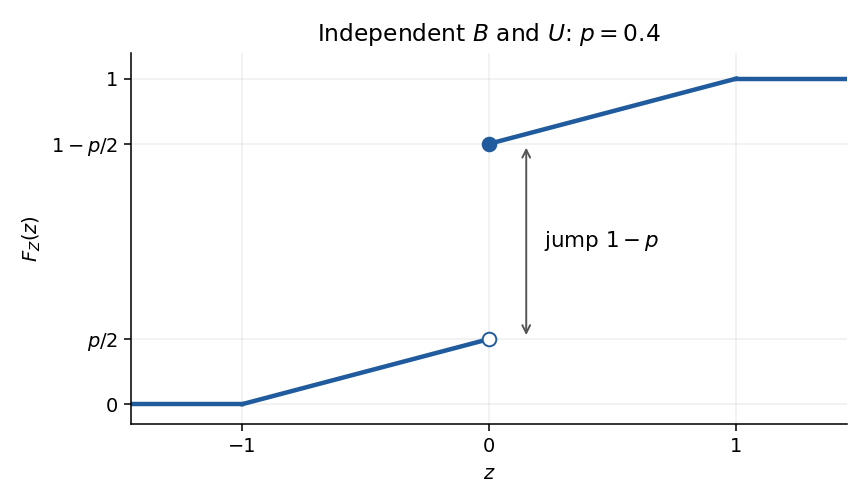
Cumulative distribution function of the independent Bernoulli-uniform product, illustrated at
. Details. 
Under the literal assumptions, write . The general answer is , so the continuous part of the sketch is undetermined. The jump at zero is still exactly , because . In the dependent counterexample from (ii), for , for , and for .
Fix and choose , independently of , with the normal distributionThe linear combination of independent normal random variables is normal. Its expected value is and its variance is . Hence for every , proving that every specified normal distribution is a self-decomposable distribution.
Fix . Since , . Using independence of random variables and the Tonelli theorem for the positive exponential integrands gives the extended-real identityThe left side is finite and the first factor is finite and strictly positive. Consequently is finite andThe same reasoning applies to , so their moment-generating functions are finite and equal throughout . The uniqueness theorem for moment-generating functions yieldsThis proves uniqueness of a self-decomposition remainder while also checking the required finiteness; no independence between and is needed.
For , integration gives for . For , the candidate remainder moment-generating function isThis is the moment-generating function of the mixture distributionConstruct it by taking an exponential random variable of rate and a Bernoulli random variable with , with mutually independent, and setting . Then is independent of , andon a neighborhood of zero. By the uniqueness theorem for moment-generating functions, , so the exponential distribution is a self-decomposable distribution.
For independent and identically distributed random variables , the linear combination of independent normal random variables has expected value zero and variance . ThusThis is exactly the requested -stability. The paper's definition is a strictly stable distribution, since it allows no centering term.
First take integers . For independent copies of , defineThe two blocks involve disjoint families of independent random variables, so and are independent. The assumed strictly stable distribution gives , , andTherefore, on any fixed probability space carrying and an independent copy , their joint probability distribution givesNow fix an arbitrary and choose rationals tending to . Continuity of the real powers gives, on that fixed probability space,The left sides all have the probability distribution of . Since almost sure convergence implies convergence in distribution, their limit has that same probability distribution. HenceThis proves strict stability implies self-decomposability. The limit argument uses no moment-generating function or finite moments, which is essential for general stable distributions.
A probability distribution on the countable state space is precisely a row vector satisfyingA transition matrix is a stochastic matrix, meaningEvery row therefore gives the conditional probability distribution of the next state given the present state. These conditions do not require to be an invariant distribution of .
The assumed identities are the detailed balance equations. Summing over and using the row sums of the transition matrix gives, for every ,All summands are nonnegative, so these countable sums are justified. Thusand is an invariant distribution.
For the countable-state Markov chain ergodic theorem, let the Markov chain be irreducible and positive recurrent, with its unique stationary distribution . From any initial state, for every real satisfying ,In particular, almost surely. This time-average conclusion requires no aperiodicity.
The countable-state Markov chain convergence theorem adds the hypothesis of an aperiodic Markov chain and concludesIt also follows that for every initial probability distribution . For an irreducible recurrent chain, the occupation-frequency theorem can also be stated as a limit , interpreted as zero for a null recurrent state; in the positive recurrent case this equals .
Under the specified evolution rule, conditional on the entire history, the next event's probability distribution depends only on the current population size. This is the time-homogeneous Markov property. Birth and immigration both increase the size by one, while death decreases it by one. Writing , the transition probabilities on areand all other entries are zero. In particular and . The row sum is . Every neighboring pair communicates, so this is an irreducible Markov chain, specifically a birth-death-immigration jump chain.
We use the stationary weights of a reflected birth-death chain, also verifying why they decide the question. If a stationary distribution exists, its equation at zero is . At , stationarity givesThus the edge flow is constant, and its value at the boundary is zero. Every stationary distribution must therefore satisfy detailed balance on each edge. Since irreducibility forces , it must be proportional toConversely, if , normalizing these positive weights gives a probability distribution satisfying detailed balance, hence a stationary distribution. Existence of a stationary distribution for an irreducible Markov chain on a countable state space is equivalent to positive recurrence.
The ratio isFor , the limit is less than one, so the ratio test gives summability. For , observe that , whereas . Thus for every , so the weights cannot be summable. This also resolves without making an inconclusive appeal to the limiting ratio. Therefore
Assume , and put and . The detailed balance equations giveMultiplying from to , the last factor telescopes, while the product involving is evaluated by the Gamma function:Consequently the requested invariant distribution can be expressed using the paper's power series asThe assumed convergence of ensures that this normalization is finite and positive.
For an explicit normalizing constant, the binomial series givesThe termwise differentiation of a power series is valid for , soThe last equality uses and : . ThereforeThese positive terms sum to one and satisfy the detailed balance equations, so part (a)(ii) verifies stationarity. Irreducibility makes the invariant distribution unique.
Every step changes the population by one, so has the parity of when . Hence . A return in two steps has positive probability from every state, and all return times are even, so the period of a state in a Markov chain is exactly two.
Each transition exchanges the even and odd classes. Since is an invariant distribution, their masses are equal: . The chain sampled at times , restricted to the even states, is irreducible and positive recurrent, and it is aperiodic because its diagonal entries are positive. Its stationary distribution is on even . The countable-state Markov chain convergence theorem applied to this sampled chain yieldsSince , the full sequence has no limit. Its time average nevertheless tends to by the countable-state Markov chain ergodic theorem.
Let count immigration events during the first transitions, and let count upward steps during those transitions. Write for the conditional immigration probability. If is the indicator that transition to is immigration, then is a bounded martingale difference with respect to the history that records event types as well as population sizes. The strong law for martingales with bounded increments impliesSince is bounded, the countable-state Markov chain ergodic theorem givesApplying the same argument to upward-step indicators gives almost surely. To evaluate this denominator, sum detailed balance over all neighboring edges:Since and , both sums equal . The denominator limit is positive, so division is valid and the immigration fraction among upward steps isThis is the requested answer in terms of . Substituting part (iii) additionally gives , so the fraction simplifies to .
Articles by others on the same topic
There are currently no matching articles.