Past exam of the statistics course of the University of Oxford / 2014 (A9, 4328)

Source: Mathematics Part A release, member FOI-20210708-1 - Data/4328.pdf, dated 25 June 2014. All twenty source leaf parts are answered below.

Bounded exact-paper checks found no matching advertisement of worked answers. The department's release policy guarantees even-year releases back at least to 2016 without specifically establishing availability for 2014; the linked answer archive redirects to Oxford SSO. No source part is skipped.

Write $I_1(\theta )$ for the Fisher information in one observation:Under the stipulated regularity assumptions, the maximum-likelihood estimator is consistent and has asymptotic normality:Equivalently, its large-sample normal approximation has mean $\theta$ and variance $1/[n{I}_1(\theta )]$. The information for the whole random sample is $n{I}_1(\theta )$; keeping the one-observation convention explicit prevents an extra factor of $n$.

Let $z={\Phi }^{-1}(1-\alpha /2)$, where $\Phi$ is the standard normal distribution's cumulative distribution function. Statistical consistency and Slutsky's theorem allow replacement of $I_1(\theta )$ by $I_1(\hat{\theta })$:Thus the probability that this standardized estimation error lies between $-z$ and $z$ tends to $1-\alpha$. Rearranging gives the Wald confidence intervalThe coverage probability is approximate, with limiting value $1-\alpha$; it is a repeated-sampling statement about the random confidence interval.

Here the exponential distribution is parametrized by its mean, so $f(x;\theta )={\theta }^{-1}{e}^{-x/\theta }$ for $x\ge 0$ and $\theta >0$. Its log-likelihood and maximum-likelihood estimate areFor one observation, ${\partial }_{\theta }\log f=-1/\theta +X/{\theta }^2$. Since $\mathrm{Var}(X)={\theta }^2$, its Fisher information is $I_1(\theta )=1/{\theta }^2$. Consequently the estimated standard error is $\overline{X}/\sqrt{n}$, givingThis is a large-sample confidence interval, not an exact one. If its lower endpoint is negative, intersecting with the parameter space $(0,\infty )$ removes impossible values without excluding any possible true statistical parameter.

Define $R={\sum }_i(Y_i-\overline{Y}{)}^2$ and $s_Y^2=R/(n-1)$, with $n\ge 2$. The unrestricted maximum-likelihood estimates are $\hat{\mu }=\overline{Y}$ and ${\hat{\sigma }}^2=R/n$. Under the null hypothesis, maximizing the normal distribution's likelihood over the remaining variance givesbecause the cross term vanishes when ${\sum }_i(Y_i-\overline{Y})=0$. At either fitted variance, the exponential factor in the likelihood function is $e^{-n/2}$, so it cancels in the ratio:The standardized test statistic isThe sample variance $s_Y^2$ uses divisor $n-1$, whereas the maximum-likelihood estimate uses divisor $n$; this explains the $n-1$ in the final expression. Under a nondegenerate normal distribution, $R>0$ with probability one.

For fixed $n$, the likelihood ratio is strictly decreasing as $t^2$ increases. A likelihood-ratio test rejects for small $\lambda$, so its rejection rule is equivalently large $|t|$. Under the null hypothesis, the standard normal distribution and chi-squared distribution results give independent quantitiesTheir ratio therefore has Student's t-distribution with $n-1$ statistical degrees of freedom. The exact level-$\alpha$ rule isThis is precisely the two-sided Student's t-test; choosing the corresponding cutoff for $\lambda$ yields the same rejection region and the same p-value.

The equal-variance two-sample Student's t-test pools the within-group sums of squares. If $s_A^2$ and $s_B^2$ are the two unbiased sample variances, the required positive square root isFor ten observations in each group, $S^2=(s_A^2+s_B^2)/2$ and the usual unpaired reference Student's t-distribution has $18$ statistical degrees of freedom, provided the assumed independence between groups is justified.

At the conventional $5\%$ significance level, Student 1's p-value $0.72$ gives no rejection of equal mean wear, while Student 2's p-value $0.009$ gives rejection of equal mean wear. The latter also rejects at the $1\%$ significance level. More generally, compare each p-value with the prespecified level $\alpha$; no decision threshold was fixed in the data supplied.

Failure to reject does not establish equality, and a p-value is not the posterior probability that the null hypothesis is true. These two-sided p-values alone also do not identify which material has larger mean wear.

Prefer Student 2's paired analysis, because the observational units are matched pairs: two shoes exposed to the same child's activity. A paired t-test uses $Y_i=A_i-B_i$, so shared child-to-child variation is removed before estimating the standard error. The independent units are the ten pairs, giving $9$ statistical degrees of freedom under the model of independent normally distributed pair differences.

The role of covariance is explicit:With common marginal variance ${\sigma }^2$ and within-pair correlation coefficient $\rho$, the true variance of the average difference is $2{\sigma }^2(1-\rho )/10$. The independent-groups calculation ignores the covariance term and uses $2{\sigma }^2/10$. Positive within-pair association can therefore make the paired standard error much smaller, explaining how the reported p-values can differ without arithmetic mistakes. The preference follows from the paired design, not from selecting the smaller p-value. Marginal normality alone need not imply normally distributed differences; exact paired inference uses the normal-difference assumption, for example justified by a joint multivariate normal distribution.

For two simple statistical hypotheses with joint probability density functions $g_0$ and $g_1$, fix a significance level $\alpha$. A randomized statistical test $\phi (x)$ is the conditional probability of rejection given the data. Choose $k\ge 0$ and, if necessary, randomization on the equality set so thatThe Neyman-Pearson lemma says that this is a most powerful test among all tests with test size at most $\alpha$:Thus the optimal ordering rejects where the alternative-to-null likelihood ratio is largest. On null-impossible observations with $g_1>0$, the rejection probability is one. Randomization is dispensable whenever an ordinary threshold already attains the required test size.

For a random sample, write $g_j(x)={\prod }_{i=1}^{n}f(x_i;{\theta }_j)$, $j=0,1$, for its joint probability density functions. Let $\phi$ be any competing statistical test of level at most $\alpha$. Pointwise,Indeed, where $g_1>k{g}_0$, ${\phi }_{\ast }=1\ge \phi$; where $g_1<k{g}_0$, ${\phi }_{\ast }=0\le \phi$, so both factors have the same sign. On the equality set the product is zero, regardless of randomization. Integrate over the joint sample space using its ordinary volume measure:Since $k\ge 0$ and ${\mathbb{E}}_0{\phi }_{\ast }=\alpha \ge {\mathbb{E}}_0\phi$,This proves maximal power. A continuous sample distribution does not itself guarantee that the equality set of the likelihood ratio has zero probability; allowing randomization there makes the proof valid in that case too.

Put $T={\sum }_i{X}_i$. For interior parameters $0<{\theta }_0<{\theta }_1<1$, the alternative-to-null likelihood ratio isThe second base is greater than one, so this is strictly increasing in $T$. The Neyman-Pearson lemma therefore gives an upper-tail rejection rule. Under the null hypothesis, $T\sim \mathrm{Bin}(n,{\theta }_0)$, and an ordinary conservative threshold can be chosen asThere is an important discrete qualification: an integer cutoff need not have test size exactly $\alpha$. To obtain exact size, choose an integer $b$ with ${\mathrm{Pr}}_0(T>b)\le \alpha \le {\mathrm{Pr}}_0(T\ge b)$, reject certainly when $T>b$, and at $T=b$ reject with probabilityThis randomized statistical test is a most powerful test at exact size $\alpha$; when a binomial upper tail equals $\alpha$, no randomization is needed and the stated region is literal. Otherwise the unrandomized upper-tail region has size at most $\alpha$, and the exact-size result includes the boundary randomization. Endpoint parameter cases retain the same upper-tail ordering by taking limits, with ties resolved on the null-supported outcomes.

The sample mean $\overline{X}=T/n$ has mean $\theta$ and variance $\sigma (\theta {)}^2=\theta (1-\theta )/n$. The central limit theorem gives a normal approximation for interior $\theta$ when both expected binomial counts are sufficiently large. Under the null hypothesis, a level-$\alpha$ upper-tail cutoff is approximatelyTo obtain the power function, evaluate this same cutoff under the true statistical parameter $\theta$, standardizing with $\sigma (\theta )$:Here $\Phi$ is the standard normal distribution's cumulative distribution function. The formula treats the binomial threshold as continuous; exact integer cutoffs and boundary randomization are finite-sample refinements.

Here $z_{\alpha }=1.96$, $\sigma (1/2)=1/(2\sqrt{n})$ and $\sigma (3/4)=\sqrt{3}/(4\sqrt{n})$. The desired approximate power is at least $0.975=\Phi (1.96)$ exactly when the argument of the upper tail in part (i) is at most $-1.96$:Rearranging and squaring the positive quantities yieldsThis is a normal approximation to a sample size calculation. It is not a guarantee of the exact finite-sample power for an arbitrary unrandomized binomial cutoff; the discrete test size and power can instead be checked using binomial probabilities.

Given observed data $x$, a credible interval $[L(x),U(x)]$ has posterior probability $1-\alpha$:For a continuous posterior distribution with probability density function $\pi (\theta \mid x)$, this is ${\int }_{L(x)}^{U(x)}\pi (\theta \mid x)d\theta =1-\alpha$. The probability is conditional on the observed data and concerns the statistical parameter under its posterior distribution; it does not assert frequentist coverage probability.

An equal-tailed credible interval allocates equal posterior probability to its two excluded tails:For a continuous strictly increasing posterior cumulative distribution function $F$, the endpoints are $F^{-1}(\alpha /2)$ and $F^{-1}(1-\alpha /2)$.

A highest posterior density interval instead includes the parameter values of greatest posterior density: there is a cutoff $c$ such that the retained region is a superlevel set of $\pi (\theta \mid x)$, of posterior mass $1-\alpha$. Every interior retained value has density at least as large as every excluded value, apart from possible ties. For a unimodal continuous density this is an interval; when both endpoints lie inside the support they have equal posterior density. For a multimodal posterior distribution, a highest-density region may be a union of intervals, rather than one interval. Equal tail probabilities and highest density are different criteria.

Let $s={\sum }_i{x}_i$, $A=a+s$ and $B=b+n$. Conditional independence gives the Poisson distribution's likelihoodMultiply by the prior gamma distribution's density and discard factors independent of $\theta$:Normalizing with the gamma function identifiesHere $A=a+s$ is the shape and $B=b+n$ is the rate, not the scale. This is conjugate prior updating for a Poisson distribution.

The mean of a shape-rate gamma distribution is shape divided by rate. Hence the posterior mean isBoth weights are positive and sum to one. This is a convex combination of the prior mean and the sample mean, provingFor $n\ge 1$ it lies strictly between them if the two means differ, and equals both if they agree. The rate $b$ acts as the prior weight relative to the $n$ observed exposure units.

Let $F$ be the cumulative distribution function of a gamma distribution with shape $A=a+{\sum }_i{x}_i$ and rate $B=b+n$; explicitly,The posterior distribution is continuous and has positive density on $(0,\infty )$, so its quantiles give the requested equal-tailed credible interval:Equivalently, $2B\theta \mid x\sim {\chi }_{2A}^2$, so the endpoints can be written as the corresponding chi-squared distribution quantiles divided by $2B$. Either form excludes posterior probability $\alpha /2$ from each tail.

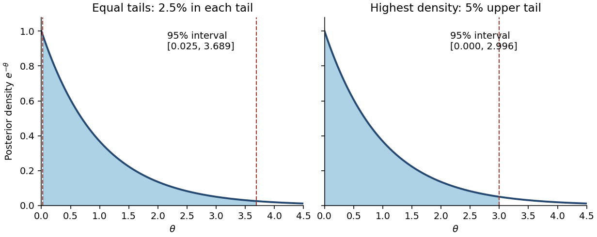
No. A permitted counterexample is $a=1$ with all observed counts zero. Then $A=1$ and the posterior distribution is an exponential distribution with rate $B=b+n$, whose density decreases strictly from the left boundary. Its equal-tailed credible interval isHere $L>0$. This excludes values just above zero whose posterior density is larger than that of retained values near $U$, violating the highest-density criterion. The actual highest posterior density interval starts at the support boundary and solves $1-e^{-Bh}=1-\alpha$:Writing zero as the endpoint causes no problem because a single point has zero posterior probability. Thus even within the gamma family the two intervals need not agree. More generally, for an interior unimodal gamma distribution, highest-density endpoints have equal densities, whereas equal-tailed endpoints need not.

Use $A=a+{\sum }_i{x}_i$ and $B=b+n$ as above. The future observation is independent of the old observations conditional on $\theta$, so the posterior predictive probability is obtained by integrating its Poisson distribution against the posterior distribution of $\theta$:The last integral is the normalizing gamma function integral, equal to $\Gamma (A+k)/(B+1{)}^{A+k}$. This is a negative binomial distribution in the count-of-failures convention with shape $A$ and success probability $B/(B+1)$; the gamma-function expression remains valid for noninteger $A>0$. As checks, its mean is $A/B$, and the law of total variance gives variance $A/B+A/B^2$. The additional term is the contribution of posterior uncertainty in $\theta$.