Use the angular coordinate for the position on the ring. The kinetic energy is . The gravitational potential energy is constant because the ring is horizontal, and the ideal constraint force has no tangential component. Thus the Lagrangian has no dependence on itself: it is a cyclic coordinate.
The Euler-Lagrange equation givesEquivalently, the conserved conjugate momentum is the vertical angular momentum, as required by rotational symmetry.
Let and be the lower and upper azimuthal angles, measured from a common fixed direction. The squared spring length isBy Hooke's law, a spring with zero natural length has potential energy . ThereforeConstant gravitational energies can be omitted. It is useful to define the moments of inertia , and the angular coupling . The part of the potential that affects motion is simply . In particular, changes the constant spring energy but not the angular equations, because the spring has zero natural length.
The two continuous, time-independent symmetries are time translation and a common rotation of both angles. Their Noether charges are respectively the total energy and vertical angular momentum:For the second symmetry, and , so the Noether theorem gives the sum of their conjugate momenta. Independent rotations are not symmetries of the spring coupling.
There are also discrete symmetries: simultaneous reflection , and time reversal in classical mechanics, which reverses both angular velocities. These leave the dynamics invariant but provide no additional infinitesimal Noether charges. Combined with common rotations, the reflections give the full planar orthogonal symmetry of the angular geometry. If , interchange of the two angular coordinates is an additional discrete symmetry of the reduced dynamics.
There is a further useful time-dependent symmetry, up to a total derivative, on a continuous lift of the angles: adding the same constant angular velocity, . It changes byIts conserved quantity is . It is the integration constant for free common rotation, rather than a new globally single-valued angle charge on the configuration torus. The globally defined continuous charges are and above.
The angular Euler-Lagrange equations areA static equilibrium point has both angular velocities zero and . Hence the complete equilibrium families, with angles taken modulo , areThe first family is aligned in azimuth and minimizes the spring length; the second is antipodal and maximizes it. Their potentials are and , respectively. Common rotations generate a whole family rather than isolated equilibria.
Let be or , and write the angular displacements as . To quadratic order the restoring potential energy is . The linearized normal mode equation isThe determinant gives . Thus the normal modes of two spring-coupled coaxial rotors areFor the aligned family, the relative mode oscillates with positive frequencyFor the antipodal family, , so that displacement has solutions and the equilibrium is unstable.
The common zero mode has . It describes a neutral displacement or uniform common rotation, not a restoring oscillation. Thus the aligned family is stable with respect to relative motion and has orbital stability modulo common rotations. A particular static point is not strictly Lyapunov stable against unrestricted small velocity perturbations: arbitrarily small nonzero eventually moves the common angle far from that point. With , the common angle is fixed and the aligned relative equilibrium point is stable. This distinguishes the symmetry-induced drift from the exponential instability of the antipodal family.
A common rotation changes neither the separation nor the spring energy. Its infinitesimal direction is , exactly the zero-frequency normal mode. Thus the continuum of rotated equilibrium points requires that zero mode; a nonzero restoring frequency in that direction would contradict rotational symmetry.
The second mode has , so it changes the relative angle while leaving the inertia-weighted common angle unchanged. It therefore carries zero perturbation in the conserved angular momentum associated with common motion. Indeed the coordinatesseparate the Lagrangian exactly:The cyclic coordinate is free, while has restoring or inverted curvature. This also explains why all members of either equilibrium family have the same frequencies. Reflection symmetry makes the potential even in , and the stable oscillatory mode is consistent with time reversal in classical mechanics through its two opposite frequency signs.
Vary the action with compactly supported , or impose vanishing and its first derivatives on the spacetime boundary. The first variation isOne integration by parts on the first-derivative term and two on the second-derivative term remove all derivatives from . The boundary terms vanish, leavingThe fundamental lemma of the calculus of variations gives the Euler-Lagrange field equation with second derivatives:Repeated indices run over time and space. The coefficient of the symmetric second derivative is defined by the displayed variation; if is instead treated as a single independent mixed derivative variable, it is counted once rather than twice.
Interpret as the small transverse displacement of the elastic beam. The first term is the positive kinetic energy density , with the mass per unit length. The Lagrangian density is kinetic minus potential energy, so the potential density encoded by the other two terms isFor a compressed rod, transverse deflection releases compression energy: the small-slope geometric change in length is proportional to , so the applied compressive load lowers the potential by . This explains the positive sign of the term in the Lagrangian. Tension would give the opposite sign and a restoring gradient term.
Bending costs elastic energy. At small slopes the curvature is , so positive bending stiffness gives potential , and hence a negative term in the Lagrangian. For a uniform slender beam is its flexural rigidity. The competition between destabilizing compression and stabilizing bending is responsible for Euler buckling of an elastic filament.
A constant shift leaves every derivative unchanged, and the density has no undifferentiated . Thus it is exactly invariant under this scalar-field shift symmetry. Localize the shift parameter temporarily to :Integrating the last term by parts once identifies the Noether current for a constant shift with second derivatives:The Euler-Lagrange field equation is , precisely the continuity equation . Therefore the conserved quantity, when the endpoint current vanishes or the field has suitable periodic/decaying conditions, isthe total transverse momentum. More explicitly . The fixed endpoints introduced later can exert transverse forces and break the global shift symmetry of the boundary problem, so vanishing endpoint current must not be inferred merely from fixed displacement.
For this density the Euler-Lagrange field equation with second derivatives givesInsert a plane wave . The second and fourth spatial derivatives give and , respectively, soFor propagating modes, and the phase velocity has magnitude , which depends on the wave number. Thus the waves are dispersive. For , the squared frequency is negative: the corresponding solutions grow or decay exponentially rather than propagate with a real frequency. The uniform displacement is a zero-frequency shift mode.
The dispersion relation shows that an infinite rod has unstable long-wave modes. A finite rod excludes sufficiently long wavelengths, so stability depends on its length and the precise end conditions. The fourth spatial derivative requires two conditions at each end; fixing transverse positions alone does not specify whether slopes are constrained.
First take displacement-fixed ends with free rotation. Setting leaves slope variations free; the bending boundary term in the first variation then gives the corresponding natural boundary conditions on the slope, . The spatial normal modes are , andThe first mode destabilizes first. ConsequentlyAt equality, the first mode has zero restoring force and is marginal, with a static component and a possible linear-in-time component in the linear theory. Every integer gives an exponentially growing mode.
If "fixed" instead means clamped, the clamped boundary condition is at both ends. The critical compression is thenFor example, the static critical shape obeys the four clamp conditions and the zero-frequency equation at this load. To establish that it is the first threshold, write : it has zero endpoints and zero mean, and periodic extension gives by the zero-mean periodic Poincaré inequality, with equality at . This proves the critical Rayleigh quotient. Both cases are instances of the compressed Euler-Bernoulli beam and its endpoint-dependent buckling threshold. The source does not specify the endpoint rotation, so both interpretations are stated explicitly.
The mean-field approximation replaces the fluctuating environment of each microscopic variable by a uniform average field. For spins, write and drop products between different sites. The resulting single-site problem can be solved independently, and its average spin must reproduce the assumed order parameter : this is the self-consistency equation.
It is reliable when correlated thermal fluctuations about the mean are small, for example with many interacting neighbours, long-range interactions or high spatial dimension. Near a thermodynamic critical point the quantitative test is the Ginzburg criterion. For short-range scalar ordering the upper critical dimension is four, with logarithmic qualifications at four; a two-dimensional nearest-neighbour lattice is below this and its asymptotic critical region of a phase transition is not described accurately by simple mean-field theory.[ref]
Statistical Field Theory by David Tong. §2.2.4, The Upper Critical Dimension: correlation-volume fluctuations and the Ginzburg criterion
The square lattice has coordination number of a lattice . The mean-field decoupling isAccounting for the factor in the directed-neighbour sum gives the Hamiltonian in the mean-field approximation:The constant term is necessary to correct the double counting of the interaction. Let . The one-site partition function isso . The Helmholtz free energy is thereforeThe equilibrium mean-field approximation is obtained by minimizing this expression over the allowed . The state supplies the extra in ; omitting it would instead describe the two-state Ising model. This is the Blume-Capel mean-field transition at zero single-ion anisotropy.
The self-consistency equation requires that the mean spin computed using the single-site Boltzmann distribution equals the spin used to form the effective field. With ,ThusEquivalently, differentiating part (b) gives , so stationarity of the Helmholtz free energy in the mean-field approximation is exactly this condition. Among multiple stationary points one must select the stable minimum.
At zero field, write the right-hand side of the self-consistency equation as , with . The origin is always a solution, and the slope there isThe critical crossing occurs when this equals one, givingThis is a continuous phase transition in the mean-field approximation. For ,so the positive branch is a strictly concave function, while is odd and bounded by one. For , the slope at zero is at most one and strict concavity puts below for every , leaving only the unmagnetized solution. For , it initially lies above but has ; hence there is one positive intersection and, by spin inversion symmetry, one negative intersection.
The curvature of the Helmholtz free energy in the mean-field approximation is per site. It is negative at below and positive at the nonzero intersections, identifying the ordered minima and the unstable zero solution.
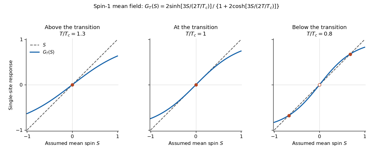
The self-consistency equation develops two nonzero order parameter branches below the mean-field critical temperature
. Details. 
The critical temperature and branches here belong to the mean-field approximation. In the exact finite system, spin inversion symmetry forces zero average magnetization at zero field; selecting a broken-symmetry phase requires the thermodynamic limit with a vanishing field of specified sign.
The small-argument Taylor series of the single-site response isLet . For a small nonzero order parameter at zero field, the self-consistency equation becomesSince and , where , this givesConsequentlyThe positive branch is the expression printed in the question, while its negative partner is required by spin inversion symmetry. The square-root behavior gives the mean-field critical exponent for the spontaneous magnetization.
The coarse-grained order parameter is a real scalar field because the microscopic spin has one component. At , spin inversion symmetry takes , so an analytic local Landau free energy contains only even powers. Near a continuous phase transition, the quadratic coefficient changes sign linearly, represented by with . A positive quartic coefficient stabilizes the density when the quadratic term becomes negative, giving the two minima below .
The ferromagnetic interaction favours neighbouring spins pointing alike, so spatial variation costs energy; its leading long-wavelength form is the positive gradient term . The source term favours alignment with the applied magnetic field and explicitly breaks spin inversion symmetry at fixed nonzero . Finally is the spin-independent background free-energy density.
The quartic sign can also be checked from part (b): its expansion containswhose quartic coefficient is positive. This is consistent with the proposed Landau-Ginzburg theory, not a tricritical truncation requiring a stabilizing sixth-order term. The microscopic square lattice is two-dimensional; the written gradient describes a profile depending on one coordinate. For general profiles, replace it by .
For a homogeneous saddle-point approximation define . With the cubic source coupling, minimizing the Landau free energy givesIts curvature is positive, so there is a unique local minimum and global minimum. The solution near hasbecause substituting this leading term makes the cubic self-interaction of order . Therefore the cubic source coupling and third-order susceptibility giveThus the first nonzero response diverges like from above. The factor is essential: the coefficient of is not itself the third derivative. This is susceptibility to the specified cubic source variable, rather than the usual third-order response to a linearly coupled field.
Apply the linear transformation of the scalar fields to either time- or space-derivative product. Its coefficients become multiplying the square of the first derivative, multiplying the square of the second, and multiplying their cross product. Invariance for arbitrary fields therefore requiresThe complete real solution isThere are four connected components, distinguished by the diagonal/antidiagonal choice and the sign of . Only the positive diagonal family is in the identity component; write to obtain , . This is the reciprocal rescaling symmetry of two cross-coupled scalar fields. The antidiagonal transformations exchange the fields as well as rescale them.
The infinitesimal connected internal symmetry of a classical field theory is , . For this exact invariance of the Lagrangian density, the Noether current is . In coordinates it isVarying the two fields gives the two wave equations and . Direct differentiation cancels the first-derivative cross terms:The Noether charge is constant when the spatial boundary flux vanishes. The disconnected transformations from part (a) do not have independent infinitesimal generators of this type.
Use coordinates , and first compute the mixed canonical stress-energy tensor supplied by spacetime translations:Define the energy density and . Direct substitution givesThe two wave equations implyFor example, differentiating and replacing each by gives exactly by the product rule. These are respectively the two component equations , establishing stress-energy conservation explicitly.
If the given metric is used to raise the second index in these unrescaled coordinates, the result is , still conserved. To display the symmetric relativistic form with light speed , choose , instead. With , the corresponding tensor isThis states the coordinate convention explicitly rather than setting in some components but not others.
The velocity coupling changes the momenta and the undifferentiated field terms. Variation with respect to gives the equation for :so the two Euler-Lagrange field equations areThey describe damped and antidamped fields from an antisymmetric velocity coupling. With the convention , their characteristic equations areThus the dispersion relations and modes areFor each spatial Fourier mode, the general solution is the linear combination of its two temporal branches; spatial superposition gives the general field. Take real parts or suitable complex conjugate pairs to obtain the required real fields. At the repeated-root threshold, the independent second temporal solution contains an extra factor , as detailed next.
Above the threshold, , the square root in part (d) is real. Both fields oscillate, but the first has envelope and the second . Thus the first is damped and the second amplified.
Below the threshold, set . The temporal factors areThey are nonoscillatory. For nonzero , , so both first-field branches decay and both second-field branches grow. At , one branch is constant; the other is for or for .
At equality, the repeated temporal root gives for the first field and for the second. The full two-field system is generically unstable on both sides because of the amplified sector. This is compatible with its autonomous Lagrangian: the total conserved energy is an indefinite quadratic form, rather than a positive energy forcing every component to remain bounded.
Articles by others on the same topic
There are currently no matching articles.