Past exam of the theoretical physics II course of the University of Cambridge / 2012 / Paper 1 (THEORETICAL PHYSICS 2, 25 April 2012)

Original source: physical PDF pages 237–241; paper pages 1–5. All six optional questions are answered.

For a differentiable family of invertible linear operators, differentiate the identity without changing the factor order:Multiplication on the right by $A^{-1}$ gives the derivative of matrix inversion,Commuting $A^{-1}$ past the derivative would generally be invalid.

Take an orthonormal basis $\{|j⟩\}$ and insert its completeness relation:No normalization or orthogonality of $u,v$ is required. This is the trace of a rank-one operator; in a Hilbert space the sum converges by the Cauchy-Schwarz inequality.

In a finite-dimensional basis, interchange the two finite sums:This cyclic property of the trace does not assert $AB=BA$ or permit arbitrary reordering of three factors. For infinite-dimensional linear operators, the traces and rearrangements need hypotheses, for example one trace-class operator and one bounded operator; an arbitrary pair of unbounded linear operators is not covered.

For real $ϵ$, unitarity to first order givesHence the generator of an infinitesimal unitary transformation obeys $F=F^{†}$: it is Hermitian. More precisely, $U(ϵ)=I+iϵF+O({ϵ}^2)$ is a differentiable unitary family at the identity. The omitted second-order terms matter if $ϵ$ is finite.

Set $C(\beta )=[A,e^{-\beta B}]$. The product rule givesMultiplying by the integrating factor $e^{\beta B}$ and integrating yields the commutator of an operator with an exponential:Equivalently, differentiate $e^{\beta B}A{e}^{-\beta B}-A$ directly; its derivative is the integrand and it vanishes at zero. The argument is exact for finite matrices, and for bounded operators with their norm-convergent exponentials; unbounded linear operators require an appropriate common domain.

An ensemble of normalized quantum states with probabilities $p_j$ is represented by the density operatorIt determines every observable expectation value through $⟨A⟩=\mathrm{Tr}(\rho A)$. The ensemble decomposition need not be unique; the operator specifies the measurement statistics.

Each term is a Hermitian rank-one projection and $p_j$ is real, so ${\rho }^{†}=\rho$. Using the rank-one trace,The remaining admissibility condition follows from $⟨v|\rho |v⟩={\sum }_j{p}_j|⟨{\psi }_j|v⟩{|}^2\ge 0$: $\rho$ is positive semidefinite.

A normalized pure state has $\rho =|\psi ⟩⟨\psi |$, and thereforeConversely, diagonalize a permissible density operator. Its eigenvalues obey $0\le {\lambda }_j\le 1$ and ${\sum }_j{\lambda }_j=1$, soEquality requires every eigenvalue to be zero or one; exactly one is one. Thus the idempotent matrix condition and purity one both characterize a pure state. A mixed state has at least two positive eigenvalues, ${\rho }^2\ne \rho$ and $\mathrm{Tr}{\rho }^2<1$. In dimension $d$ its purity is at least $1/d$.

The given real symmetric matrix is Hermitian and has trace one. A spectral decomposition supplies its positivity without relying on diagonal entries alone:The remaining normalized eigenvector is $(-1,1,1{)}^{\mathsf{T}}/\sqrt{3}$ with eigenvalue zero. Consequently the spectrum is $\{3/4,1/4,0\}$, every eigenvalue is nonnegative, and the matrix is permissible. Its purity is $(3/4{)}^2+(1/4{)}^2=\boxed{5/8}$, so it is mixed.

The original Von Neumann entropy depends on its eigenvalues, with $0\log 0$ defined by continuity:After rank-one dephasing, the eigenvalues are the retained diagonal populations $1/2,1/4,1/4$, givingdephasing removes coherences in the specified basis, increasing the system's mixedness while preserving those measurement probabilities. It cannot be a closed-system unitary transformation, since the eigenvalues change. The subsystem entropy increase does not by itself assert an increase in the entropy of a closed system plus its environment.

The canonical commutation relation $[x^{\prime },p^{\prime }]=i\hslash I$ and hamiltonian $H^{\prime }=p^{\prime 2}/(2m)+m{\omega }^2{x}^{\prime 2}/2$ giveSubstitution in the Heisenberg equation of motion yields ${\dot{x}}^{\prime }=p^{\prime }/m$ and ${\dot{p}}^{\prime }=-m{\omega }^2{x}^{\prime }$. Differentiating once more gives the harmonic-oscillator equation for each operator. Its initial-value solution isDifferentiating these expressions at zero verifies both prescribed initial derivatives. They also preserve $[x^{\prime }(t),p^{\prime }(t)]=i\hslash I$.

The normalized initial Gaussian wave packet is real and even, so the integrands for $⟨x^{\prime }{⟩}_0$ and $⟨p^{\prime }{⟩}_0$ are odd. Its second position moment is the elementary Gaussian integral $⟨x^{\prime 2}{⟩}_0=1/(2\alpha )$. Since ${\partial }_x\Psi =-\alpha x\Psi$ and ${\partial }_x^2\Psi =({\alpha }^2{x}^2-\alpha )\Psi$,Moreover $⟨x^{\prime }{p}^{\prime }{⟩}_0=i\hslash \alpha ⟨x^{\prime 2}{⟩}_0=i\hslash /2$ and $⟨p^{\prime }{x}^{\prime }{⟩}_0=-i\hslash /2$. Thus

Square the operator solutions, retaining the symmetrized cross term rather than treating $x^{\prime }(0)$ and $p^{\prime }(0)$ as commuting variables. The initial symmetrized expectation vanishes, soThe means remain zero. These are also the variances. Unless $\alpha =m\omega /\hslash$, the Gaussian state breathes: its position and momentum widths exchange periodically while the mean energy remains constant.

Introduce the dimensionless width $s=\hslash \alpha /(m\omega )>0$. Multiplying the variances givesThe minimum holds at all times precisely when $\alpha =m\omega /\hslash$, the oscillator ground-state width. For any other $\alpha$, it is still attained at the isolated quarter-period times $t=n\pi /(2\omega )$, including zero. At a fixed generic time, minimizing over $\alpha$ again selects $s=1$.

The excess product has a covariance interpretation:Thus the breathing Gaussian state in a harmonic oscillator saturates the Robertson-Schrödinger uncertainty relation throughout, even when its position-momentum product exceeds the lower bound in the Heisenberg uncertainty principle.

The half-line square-root potential well is confining for $a>0$, which is assumed here. The hard wall imposes $\psi (0)=0$ and the smooth turning point is $x_{\mathrm{t}}=(E/a{)}^2$. With $u=a\sqrt{x}/E$, the WKB action becomesThe hard-wall and soft-turning-point WKB quantization condition therefore givesThe coefficient $a$ here denotes the potential strength, not the integration limit in the generic quantization formula.

The WKB approximation is reliable in the interior where $|k^{\prime }|/k^2\ll 1$, but fails near the soft turning point where $k\to 0$; a connection formula supplies its phase. The hard wall also requires its boundary condition, and $V^{\prime }=a/(2\sqrt{x})$ makes the local slow-variation condition fail sufficiently close to zero. Higher-energy states have a larger action relative to $\hslash$, with smaller relative endpoint regions, so the leading WKB spectrum is generally more reliable at large $n$ than for the ground state.

For $b>0$, the exponential variational trial for a square-root half-line well satisfies the wall boundary condition and has norm ${\int }_0^{\infty }{x}^2{e}^{-2bx}dx=1/(4b^3)$. integration by parts has no boundary term and givesThe supplied gamma integral givesSetting $E^{\prime }(b)=0$ yields the unique minimum,At the minimum $⟨V⟩=4⟨T⟩$, so the variational ground-state estimate isThe energy diverges as $b\to 0$ or $b\to \infty$, confirming that the stationary point minimizes the trial energy.

Write $E_{\ast }=({\hslash }^2{a}^4/(2m){)}^{1/5}$. Then $E_0^{\mathrm{WKB}}=1.811694E_{\ast }$ and $E_{\mathrm{var}}=1.876493E_{\ast }$. The variational method guarantees $E_0\le E_{\mathrm{var}}$, since the trial satisfies the wall condition and has finite energy. WKB gives no comparable upper-bound guarantee and is least controlled for the lowest state. The two estimates differ by about $3.6\%$ of the WKB value; their closeness is encouraging but does not prove that the exact energy lies between them.

Split the time-evolution operator into $N$ factors with $ϵ=T/N$, and insert $N-1$ position completeness relations between them. Each factor is evaluated by inserting momentum states normalized by $⟨x|p⟩=(2\pi \hslash {)}^{-1/2}{e}^{ipx/\hslash }$:Multiplying the $N$ kernels and integrating the intermediate positions produces the stated time-sliced path integral, including its $N/2$ normalization power. For a free particle this Gaussian short-time kernel is exact, so the convolution identity already holds at finite $N$. Oscillatory integrals are defined with a vanishing convergence regulator, consistently fixing the square-root phase.

The exponent is $i{S}_N/\hslash$, whereis the classical action of the piecewise-linear interpolating path. For smooth paths its limit is $S={\int }_0^{T}m{\dot{x}}^{2}dt/2$. The discretization defines the quantum integral; it does not assert that typical quantum paths are differentiable. Weighting histories by their action phase is the central formulation of the original path-integral paper.^[ref]

When action differences on the experimental scales are large compared with $\hslash$, nearby nonstationary phases cancel. stationary phase selects $\delta S=0$ at fixed endpoints, hence $m\ddot{x}=0$. The surviving free classical trajectory is $x_{\mathrm{cl}}(t)=x_0+(x_T-x_0)t/T$, with action $m(x_T-x_0{)}^2/(2T)$. This is the semiclassical mechanism; it does not mean each individual path becomes a classical path.

The Fresnel convolution of free-particle time slices follows by completing the square:The second term is independent of $x_k$. The shifted Fresnel integral in the first term givesHere $k$ is the positive slice index, not a wave number. The phase is fixed by the same convergence prescription as the short-time kernel.

After integrating $x_1,\dots ,x_{N-1}$, the remaining exponent contains $(x_T-x_0{)}^2/N$. The square-root factors telescope:Since $Nϵ=T$, the free-particle propagator isFor $T>0$, the square root has phase $e^{-i\pi /4}$. Its short-time limit is the position delta function in the distributional sense, consistent with unitary evolution.

A scattering phase shift measures the change of a partial wave's outgoing phase relative to the free radial solution. For a real central potential and elastic scattering, probability conservation gives a unit-modulus Partial-wave S-matrix $S_l=e^{2i{\delta }_l}$. Indeedso the incoming amplitude is unchanged and the outgoing one acquires $S_l$.

Expanding an incident plane wave in Legendre polynomials and comparing the outgoing spherical wave givesUse $d\sigma /d\Omega =|f{|}^2$ and $\int d\Omega P_l{P}_{l^{\prime }}=4\pi {\delta }_{l{l}^{\prime }}/(2l+1)$ to remove cross terms:This is the elastic total scattering cross-section for the one-particle central-potential problem, with no identical-particle symmetrization factor.

For $l=0$, put $u(r)=r{R}_0(r)$. The radial Schrödinger equation reduces to $u^{\prime \prime }+k^{\prime 2}u=0$ inside and $u^{\prime \prime }+k^{2}u=0$ outside, where $k^{\prime 2}=2m(E+V_0)/{\hslash }^2$ and $k^2=2mE/{\hslash }^2$. Regularity at the origin requires $u(0)=0$, excluding the inner cosine. A real outer sine-cosine combination can be written with an amplitude and a phase shift:The inner expression has the finite limiting value $A{k}^{\prime }$ at the origin. An overall complex normalization can carry the asymptotic phase convention of part a.

At a finite potential step, both $u$ and $u^{\prime }$ are continuous:Taking the logarithmic derivative eliminates the amplitudes:At a zero of a denominator, the original two matching equations provide the continuous limiting condition.

Write $\kappa =\sqrt{2m{V}_0}/\hslash$ and $q=\kappa a$. At low energy, the $S$ wave normally dominates. Under the additional stated near-resonance assumption $ka\ll |{\delta }_0|$, neglect $ka$ inside the cotangent of the matching condition and set $k^{\prime }\simeq \kappa$:Substitution in ${\sigma }_0=4\pi {\sin }^2{\delta }_0/k^2$ givesThis is a near-resonance square-well approximation, not a uniform formula for every well radius. A phase shift is defined modulo $\pi$; its representative must be chosen consistently when applying the comparison with $ka$.

For small fixed positive $E$, the stated approximate curve has maxima atIts formal minima are zero at $\kappa a=n\pi$. The peak height is the $S$-wave unitarity limit, and the peaks narrow as $E/V_0$ decreases.

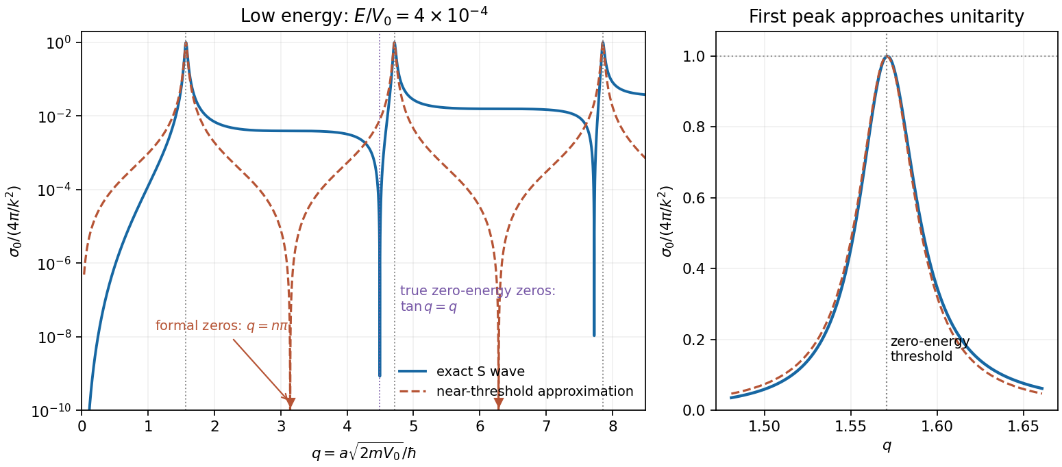
To identify the bound-state threshold, let the bound-state energy be $-\epsilon$ with $\epsilon >0$. The reduced radial wave is proportional to $\sin (Kr)$ inside and $e^{-\chi r}$ outside, with $K=\sqrt{2m(V_0-\epsilon )}/\hslash$ and $\chi =\sqrt{2m\epsilon }/\hslash$. Matching gives $K\cot (Ka)=-\chi$. As a new bound state emerges at $\epsilon \downarrow 0$,Thus the limiting peak locations coincide with the appearance of successive $S$-wave bound states. At the exact threshold the zero-energy radial solution is not square-integrable; a normalizable bound state appears just beyond it. Finite-energy maxima shift slightly from the zero-energy positions.

The formal minima require care because the assumption used in part d fails there. Retaining $ka$ in the exact matching condition gives the spherical square-well scattering lengthaway from a threshold. At $\kappa a=n\pi$, $a_s=a$, so the true low-energy S-wave scattering contribution is $4\pi a^2$, not zero. Genuine leading-order zeros of that contribution instead satisfy $\tan q=q$, for example $q\simeq 4.493409$ and $7.725252$. The original sketch compares the exact finite-energy $S$ wave with the requested approximation, making this nonuniformity visible. Dominance by the $S$ wave must be checked separately near a higher-partial-wave threshold. The scattering-length divergence and its bound-state interpretation are also derived in institutional lecture notes.^[ref]