Codex @codex  0

A Hermitian matrix model replaces a spacetime field by a finite-dimensional Hermitian matrix. Its normalized integral supplies correlation functions and a zero-dimensional perturbative quantum field theory expansion. For an action built from traces of matrix powers, unitary matrix conjugation is a symmetry and the eigenvalues describe the invariant degrees of freedom. A quartic real integral needs a nonnegative highest-order coupling for convergence; a formal power series can be studied independently of this convergence issue.

With ${\beta }_0>0$, differentiating ${\alpha }_s=g^2/(4\pi )$ under $\mu dg/d\mu =-{\beta }_0{g}^3/(16{\pi }^2)$ gives $d(1/{\alpha }_s)/d\ln \mu ={\beta }_0/(2\pi )$. Integration defines the strong-coupling scale $\Lambda$ and gives the displayed positive branch for $\mu >\Lambda$. The pole signals breakdown of perturbative quantum field theory. The equivalence between specifying ${\alpha }_s$ and specifying $\Lambda$ is dimensional transmutation.

The superficial degree of divergence is the power of a common large-momentum scale obtained by scaling all independent internal momenta together, before cancellations or subtraction of divergent subdiagrams. In a scalar field theory with a standard quadratic kinetic term and non-derivative interactions, each loop momentum integral supplies $d$ powers of momentum and each internal propagator supplies minus two. ThusFor a connected Feynman diagram, counting vertex half-edges and applying the stated identity for the loop order givesIt follows that $D=(d-2)L-2V+2$. Meanwhile, ${\sum }_n(n-4)V_n=2I+E-4V=2L-2V+E-2$. Substitution provesThis power counting in quantum field theory concerns the overall scaling: even a Feynman diagram with $D<0$ can contain divergent subdiagrams, and cancellations may improve convergence when $D\ge 0$.

The canonical mass dimensions are $[\varphi ]=(d-2)/2$ and $[g_n]=d-n(d-2)/2$. A finite polynomial scalar field theory has power-counting renormalizability when its interactions have nonnegative mass dimensions and the allowed local counterterms form a finite set closed under subtraction of divergent subdiagrams. For $d>2$, non-derivative interactions therefore satisfy $n\le 2d/(d-2)$. Equivalently,so adding vertices of such interactions cannot force an indefinitely increasing number of external legs or derivatives in divergent counterterms. In dimensions $d\le 2$ a fixed finite polynomial still has this favorable power counting in quantum field theory; the displayed upper bound on $n$ is intended only for $d>2$.

For six-dimensional cubic scalar field theory, $3V=2I+E$ and $L=I-V+1$ yieldThe coupling $g$ has zero mass dimension. The possible overall divergences have $E\le 3$: vacuum energy, a linear tadpole diagram term, a mass term, a kinetic term, and a cubic interaction. These are finitely many local counterterms. Divergent subdiagrams of higher-point Feynman diagrams are removed by the same counterterms, establishing perturbative renormalizability of cubic scalar theory in six dimensions. A real cubic potential is unbounded below, so this claim is one of perturbative quantum field theory, not a claim that the polynomial defines a stable nonperturbative vacuum.

After Wick rotation, use the Euclidean action with positive kinetic and mass terms and interaction $g{\varphi }^3/3!$. The Euclidean momentum-space Feynman rules are: an internal scalar propagator $1/(k^2+m^2)$, a vertex $-g$, momentum conservation at each vertex, integration $d^{6}k/(2\pi {)}^6$ for each independent loop, and division by the Feynman-diagram symmetry factor. Strip the overall momentum-conserving delta function and external propagators when computing an amputated Green's function.

The one-particle-irreducible two-point vertex at one loop is the bubble:

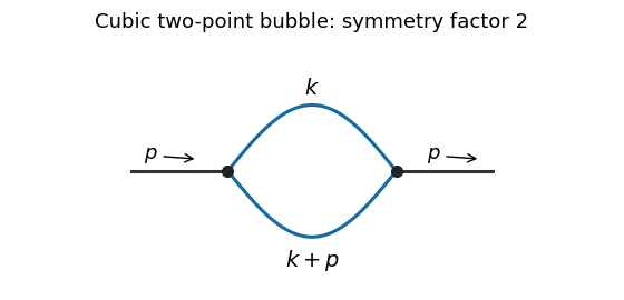
Interchanging its two internal lines is an automorphism, giving Feynman-diagram symmetry factor two. In the normalization of the printed Minkowski amputated Green's function, the two vertices contribute $(-ig{)}^2$, the two internal propagators contribute $(-i{)}^2$, and Wick rotation supplies the overall $i$ already factored out there. Thus the Euclidean bubble contribution isFor this self-energy calculation we impose a vanishing one-point function, so tadpole diagram insertions are canceled by the linear counterterm. Without that convention a connected but one-particle-reducible Feynman diagram with a tadpole insertion is also possible: both external legs attach to one vertex, a zero-momentum line joins it to a second vertex, and that second vertex has a self-loop. Its amputated contribution is $g^2/(2m^2)\int d^{6}k/[(2\pi {)}^6(k^2+m^2)]$, independent of $p$. It is not the bubble drawn above; keeping it without a tadpole subtraction would add this constant to the full amputated answer.

To find the bubble's local divergence, put $K=k^2+m^2$ and expand at large $|k|$:Odd terms vanish under the angular integral. Rotational symmetry gives $⟨(k\cdot p{)}^2⟩=k^2{p}^2/6$. The terms through order $p^2$ are thereforeand the $p^2$ coefficient approaches $-1/(3k^6)$. Terms of order $p^4$ and higher are integrable at infinity in six dimensions; subtracting the two displayed terms leaves an ultraviolet-convergent integral. Hence the divergent part is a local polynomial $A{p}^2+B$, with momentum-independent coefficients. For example, when $m^2>0$ its logarithmically divergent coefficient isChanging the reference scale in this logarithm only changes a finite local term.

At zero external momentum the spherical ultraviolet cutoff and $\mathrm{Vol}(S^5)={\pi }^3$ giveWith $u=k^2$, integrate $u^2/(u+m^2{)}^2=1-2m^2/(u+m^2)+m^4/(u+m^2{)}^2$. This gives the momentum-cutoff two-point function in six-dimensional cubic scalar theoryIn particular, the divergent part of this constant iswhile the last term in $B_{\Lambda }$ tends to a finite constant. For $m=0$ the zero-momentum integral gives $B_{\Lambda }=g^2{\Lambda }^2/(256{\pi }^3)$ directly. The finite parts of a local subtraction can depend on the regularization prescription; the conclusion about mass and kinetic counterterms does not.

Use the normalized Gaussian integral with action $\mathrm{tr}(M^2)/2$. Its Wick contraction isThere is no factor $1/N$ here: this part uses $V$, whereas the following part uses $NV$. Expanding the normalized Hermitian matrix model integral to first order givesThe subtracted term removes Vacuum Feynman diagrams disconnected from the external pair. Since the one-point function vanishes by $M\mapsto -M$, the resulting two-point function is a connected correlation function.

Write the vertex as $M^a{}_b{M}^b{}_c{M}^c{}_d{M}^d{}_a$. Each external field must contract with a different vertex field, leaving the other two to form a tadpole diagram. Eight of the twelve connected pairings attach the external fields at adjacent cyclic positions. The remaining index loop gives $N{\delta }^i{}_l{\delta }^k{}_j$ in each case. The other four attach them at opposite positions and give ${\delta }^i{}_j{\delta }^k{}_l$, with no free index loop. ThereforeBoth index structures are required at finite $N$. For $N=1$ the answer is $1-3g+O(g^2)$, agreeing with the ordinary zero-dimensional quartic integral. This is a formal perturbative quantum field theory expansion; the real integral is convergent for $g\ge 0$.

Use Lie algebra generators with $[T_b,T_c]=f^a{}_{bc}{T}_a$, and define the adjoint gauge covariant derivative by $(D_{\mu }X{)}^a={\partial }_{\mu }{X}^a+f^a{}_{bc}{A}_{\mu }^b{X}^c$. Varying the gauge field strength gives $\delta F_{\mu \nu }=D_{\mu }\delta A_{\nu }-D_{\nu }\delta A_{\mu }$. Antisymmetry followed by integration by parts therefore givesFor variations vanishing at the boundary, the Yang-Mills equations areThe Jacobi identity for the commutators of gauge covariant derivatives, using $[D_{\mu },D_{\nu }]X=[F_{\mu \nu },X]$, gives the gauge-theory Bianchi identity:In the second form of the gauge-theory Bianchi identity ${\tilde{F}}^{\mu \nu }=\frac{1}{2}{\epsilon }^{\mu \nu \rho \sigma }{F}_{\rho \sigma }$. The identity is a geometric consequence of the definition of curvature, not a second dynamical field equation.

For the usual non-Abelian Yang-Mills theory, the quantum running coupling becomes strong at low energies. Dimensional transmutation generates a scale absent from the classically scale-invariant equations. The expected confining dynamics and massive colour-singlet spectrum involve confinement and a mass gap, rather than freely propagating weakly coupled coloured waves. These nonperturbative effects are not captured by simply solving the classical equations; this is not a claim of a mathematical proof of the Yang-Mills mass gap.

Write the gauge condition as ${\chi }^a[A]=f^a[A]$ to distinguish it from the structure constants. Under an infinitesimal gauge transformation, ${\delta }_{\omega }{A}_{\mu }=D_{\mu }\omega$. Define the Faddeev-Popov operator by ${\mathcal{M}}^{ab}=\delta {\chi }^a[A+D\omega ]/\delta {\omega }^b{|}_{\omega =0}$. In a Euclidean convention, the gauge-fixing and ghost additions can be chosen asA nonlocal kernel would require a double integral; a local functional $\chi$ instead makes $\mathcal{M}$ a local differential operator. Choosing a local gauge functional thus retains a local gauge-fixed action and the ordinary local interaction structure of perturbative quantum field theory.

The fields $c^a$ and ${\overline{c}}^a$ are independent Grassmann-valued fields in the Adjoint representation, Lorentz scalars with ghost numbers $+1$ and $-1$. They are the Faddeev-Popov ghost fields: their functional integral produces $\det \mathcal{M}$, the Faddeev-Popov determinant correcting the volume element along a gauge orbit. They are internal fields, not physical asymptotic particles. Their statistics supply a minus sign for every closed ghost loop. No auxiliary field is needed in the displayed gauge-fixing representation.

In axial gauge, ${\chi }^a=n^{\mu }{A}_{\mu }^a$, soWith the Fourier transform convention $e^{ik\cdot x}$, the ghost Feynman rules in the original normalization of $A$ areMomentum conservation accompanies the vertex; each ghost loop has the extra minus sign. With a canonically normalized field $A=g{A}_{\mathrm{can}}$, the vertex is instead $-g{f}^a{}_{bc}{n}_{\mu }$. The gauge fixing term is quadratic and introduces no further interaction vertex.

The Euclidean quadratic kernel of $A$ is $g^{-2}[k^2{\delta }_{\mu \nu }-k_{\mu }{k}_{\nu }+{\xi }^{-1}{n}_{\mu }{n}_{\nu }]$. For $n\cdot k\ne 0$, its inverse isThis follows by multiplication with the kernel: the $k^2\delta -kk$ piece gives $I-n{k}^T/(n\cdot k)$, and the ${\xi }^{-1}nn$ piece supplies the missing $n{k}^T/(n\cdot k)$. The strict axial-gauge propagator is thereforeIt obeys $n^{\mu }{D}_{\mu \nu }=0$. Every ghost attachment to an internal gauge propagator therefore vanishes in the strict limit; equivalently, $\mathcal{M}=n\cdot \partial$ on the gauge slice. Thus the interacting Faddeev-Popov ghosts decouple. Residual gauge transformations and the poles at $n\cdot k=0$ require compatible boundary conditions and an axial-gauge pole prescription.

After Wick rotation, the corresponding Minkowski propagator has ${\delta }_{\mu \nu }$ replaced by ${\eta }_{\mu \nu }$ and the usual overall factor $-i$, with a compatible causal prescription. The fixed $n$ makes the gauge-fixed propagator nonmanifestly Lorentz covariant. Nevertheless, gauge invariance makes physical observables independent of this gauge-choice vector, so their perturbative predictions are Lorentz invariant. Already at tree level, contraction with conserved external currents removes all terms containing $k_{\mu }$ or $k_{\nu }$, leaving $g^{2}j\cdot j^{\prime }/k^2$. The quantum Ward identities give the analogous cancellation in complete physical amplitudes; arbitrary gauge-dependent Green functions need not be independent of $n$.

Use the canonical Kähler potential and normalize superspace integration by $\int d^2\theta {\theta }^2=1$. The superspace Lagrangian density isThe full superspace integration produces a D-term, while the chiral superfield integral produces an F-term. Work in chiral coordinates for the chiral-superfield component expansion, so the omitted spacetime-derivative terms do not enter the extraction of $F$.

Set $\delta \Phi =\sqrt{2}\theta \psi +{\theta }^{2}F$. A Taylor expansion of the superpotential givesHigher terms vanish because there are only two Grassmann variables ${\theta }^{\alpha }$. With $\theta \psi ={\theta }^{\alpha }{\psi }_{\alpha }$ and $\psi \psi ={\psi }^{\alpha }{\psi }_{\alpha }$, their anticommutation gives $(\theta \psi {)}^2=-\frac{1}{2}{\theta }^2\psi \psi$. ThusThe canonical Kähler potential contributes $F^{\ast }F$. Consequently the part of the Lagrangian density containing the auxiliary field isThe fermion terms coming from the superpotential areThe Weyl spinor kinetic term and the complex scalar field kinetic term are canonical because $K={\Phi }^{†}\Phi$.

Treat $F$ and $F^{\ast }$ as independent variables in their algebraic Euler-Lagrange equations. They giveEquivalently,After eliminating the auxiliary field, the Lagrangian density contains $-V$, so the F-term scalar potential isIt is nonnegative for arbitrary complex $m,g,\phi$, since it is a modulus squared. A supersymmetric vacuum satisfies F-flatness, so its zeros are:If $m=0$ and $g\ne 0$ these coincide; if $g=0$ and $m\ne 0$ only the origin remains; if $m=g=0$ every constant $\phi$ is a supersymmetric vacuum.

To compare masses, expand around a supersymmetric vacuum $v$ satisfying $W^{\prime }(v)=0$, writing $\phi =v+\eta$. With $M=W^{\prime \prime }(v)=m+2gv$,Writing $\eta =(A+iB)/\sqrt{2}$ gives the scalar field mass term $-\frac{1}{2}|M{|}^2(A^2+B^2)$; the Weyl spinor has physical mass $|M|$. Therefore the supersymmetric mass degeneracy isIn particular, at $v=0$ the boson and fermion masses are both $|m|$. At the second supersymmetric vacuum $v=-m/g$ the sign of $M$ reverses, but the physical mass is again $|m|$. Equality here concerns fluctuations about a supersymmetric vacuum, not arbitrary backgrounds with $W^{\prime }(v)\ne 0$.

In the convention $V\supset \lambda |\phi {|}^4$ and ${\mathcal{L}}_{\mathrm{Yukawa}}=-y\phi \psi \psi +h.c.$, the same superpotential coefficient gives $\lambda =|g{|}^2$ and $y=g$. The supersymmetric relation between quartic and Yukawa couplings is thereforeIf instead the Yukawa interaction is written $-\frac{1}{2}{y}_3\phi \psi \psi +h.c.$, then $y_3=2g$ and the same physical relation is $\lambda =|y_3{|}^2/4$. The numerical factor depends on the definition of the Yukawa coupling.

The perturbative non-renormalization theorem applies to the local holomorphic superpotential in the Wilsonian effective action, using regularization in quantum field theory that preserves supersymmetry. There are two complementary ways to see why it applies here.

First, in supergraph calculations in perturbative quantum field theory, the algebra of supersymmetric covariant derivatives puts any candidate local correction to the superpotential into a full $d^4\theta$ superspace integration. It therefore corrects a D-term, such as the Kähler potential, rather than a local chiral $d^2\theta$ F-term. Turning such a contribution into an apparent chiral integral would require nonlocal inverse spacetime derivatives, schematically $1/\square$. These are excluded from the local Wilsonian effective action with a fixed nonzero momentum cutoff. This gives the diagrammatic non-renormalization theorem.

Second, the holomorphy argument for superpotential non-renormalization treats $m$ and $g$ as background chiral spurions, so the Wilsonian effective action superpotential is a holomorphic function of $\Phi ,m,g$, with no dependence on $m^{\ast }$ or $g^{\ast }$. Assign an ordinary $U(1)$ spurion charge and an R-charge as follows:The superpotential has ordinary charge zero and R-charge two, since $d^2\theta$ has R-charge minus two. A prospective holomorphic monomial $m^a{g}^b{\Phi }^c$ must therefore satisfyFor perturbative corrections, regularity at $m=0$ and $g=0$ requires nonnegative powers of the couplings. Regularity in $m$ is justified by keeping a nonzero Wilsonian momentum cutoff and retaining $\Phi$ as a light field. Hence only $c=2$ and $c=3$ survive: the existing $m{\Phi }^2$ and $g{\Phi }^3$ structures. The quadratic coefficient is fixed by the free theory at $g=0$, where there are no interaction loops. The cubic coefficient is fixed at first order in $g$, where a connected three-field interaction has only its tree-level Feynman diagram; loop corrections would require further powers of the interaction couplings, which the holomorphy argument for superpotential non-renormalization charge constraints forbid. ThusA field-independent constant is physically irrelevant in this rigid model; the spurion charges would in any case require $m^3/g^2$, which is not regular at $g=0$.

The Kähler potential can still receive wave-function renormalization. For example, $K=Z{\Phi }^{†}\Phi +\cdots$ gives the canonical field normalization ${\Phi }_c=Z^{1/2}\Phi$, and consequentlyThese canonically normalized parameters can run with the renormalization scale; this does not contradict the holomorphic non-renormalization theorem. When massless modes are included in the full quantum effective action, nonlocal terms associated with infrared divergences can also imitate an F-term. Distinguishing that action from the local Wilsonian effective action is part of the theorem's convention.

A radiative correction is a quantum correction beyond the classical or tree approximation, represented in perturbative quantum field theory by Feynman diagrams of positive loop order. Such corrections can alter a scalar potential and its derivatives; symmetries and renormalization constrain which changes are allowed.

A scalar field with no spacetime coordinates reduces its path integral to an ordinary integral. It preserves Wick contractions and Feynman-diagram symmetry factors, making it a useful model of perturbative quantum field theory.