The source cover identifies Hilary Term 2021 despite the attachment's filename. Use natural units , the Minkowski metric , and . The three-dimensional scalar field theory in 3 has two spatial dimensions and one time dimension. Results are at the stated order of perturbative quantum field theory.
The momentum space Feynman rules use the scalar propagator and two Dirac propagatorsThe cubic scalar field interaction vertex is . Each of the two flavour-changing Yukawa coupling interaction vertices, and , has factor in Dirac spinor indices. A fermion flow arrow continues through each interaction vertex, but its species changes. There is no or interaction vertex.
Every interaction vertex carries with inward four-momenta. Integrate each independent loop momentum with , divide by the Feynman-diagram symmetry factor, and include a minus sign and a gamma-matrix trace for each closed fermion loop. The is the Feynman i-epsilon prescription.
For an amputated scattering amplitude, incoming fermions supply and outgoing fermions supply ; incoming antifermions supply and outgoing antifermions supply . An external real scalar field particle supplies . Use the standard relativistic normalization of a one-particle state; the external factors belong to that normalization and the Lorentz-invariant phase-space measure, rather than an additional factor in the invariant scattering amplitude.
The original tree-level Feynman diagrams below use solid arrowed fermion lines and dashed scalar field lines. The labelled internal momenta run in the indicated directions; and label the corresponding interaction vertices.
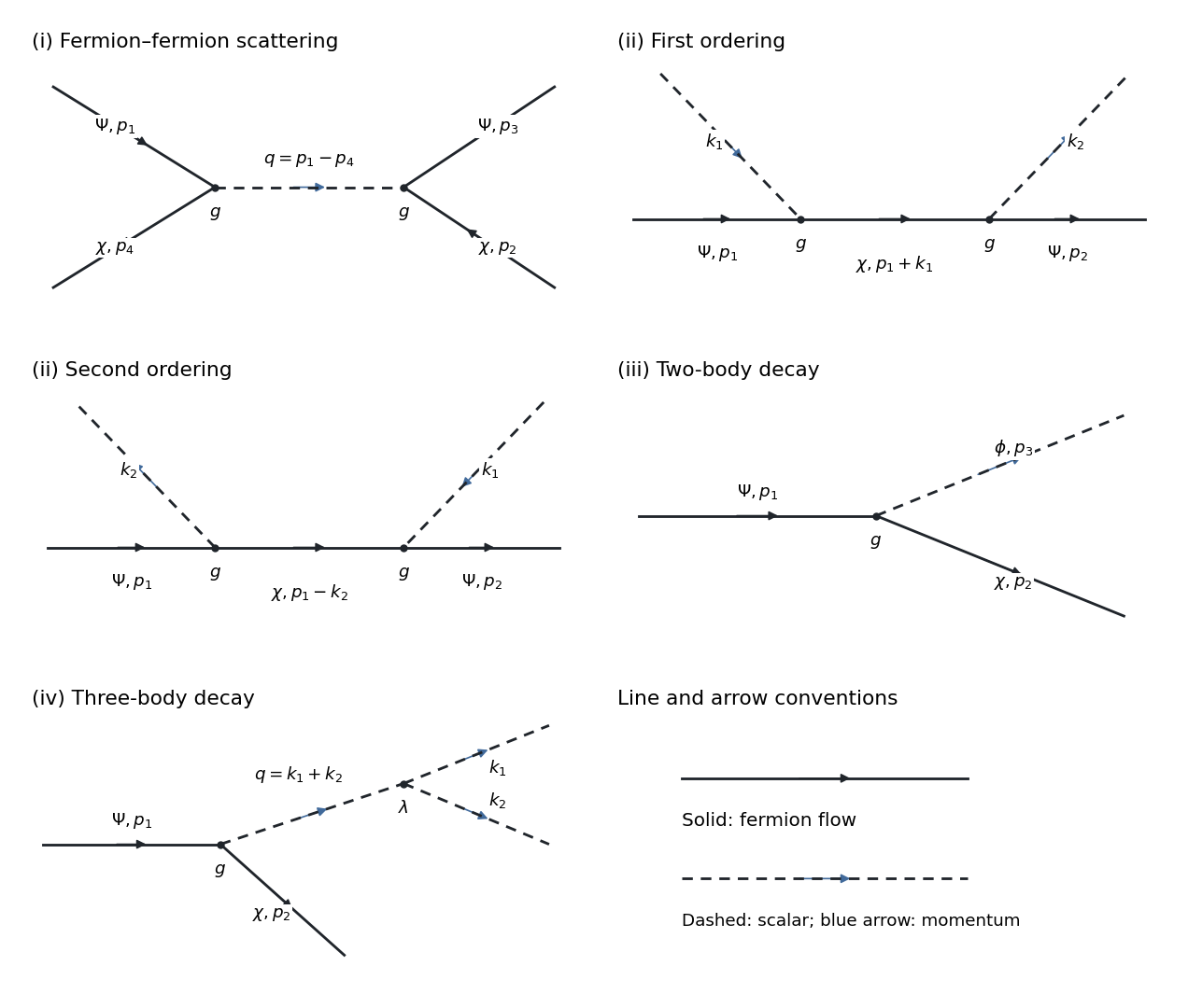
Momentum-labelled tree diagrams for the four processes; the middle row contains the two exchange orderings.
Details. 
Label the external four-momenta by . The only tree-level Feynman diagram exchanges a scalar field particle between the transitions and . Its internal four-momentum is . Thus its scattering amplitude, with a consistent external-state ordering, isIt is the crossed, or -channel, exchange with these labels. A direct -channel scalar field exchange would need a flavour-preserving Yukawa coupling, which the Lagrangian density does not contain. There is no annihilation Feynman diagram for two incoming fermions.
For , there are two tree-level Feynman diagrams, both with an internal fermion. Their internal four-momenta are and . The scattering amplitude isThese are the two possible absorption/emission orderings along the fermion flow. There is no third tree-level Feynman diagram using the cubic scalar field interaction vertex, since attaching its remaining scalar field line to the external line would require a forbidden interaction vertex.
For , the sole tree-level Feynman diagram is a single flavour-changing Yukawa coupling interaction vertex, with . Its invariant decay amplitude isThe solid arrow passes from the incoming to the outgoing ; the dashed outgoing line carries .
For , the sole tree-level Feynman diagram has a Yukawa coupling interaction vertex producing an off-shell scalar field particle of four-momentum , followed by its cubic scalar field interaction vertex. Its invariant decay amplitude isTwo successive Yukawa coupling interaction vertices would change the fermion species twice and leave a , so they cannot produce this final state. Interchanging the two identical outgoing bosons does not create another Feynman diagram; the cubic factorial is already included in the Feynman rule. The integrated decay width instead includes the identical final-state symmetry factor .
In the convention of iii, the invariant decay amplitude is . Including the common overall in the definition changes no squared decay amplitude. An unpolarized ensemble is an incoherent equal mixture of the two initial spin states; hence take a spin average over and a spin sum over the unobserved final . Different final spin states are orthogonal outcomes, so their probabilities, rather than their decay amplitudes, add.
Using the Dirac adjoint and the fermion spin sum givesThe gamma-matrix trace identities used here are and . The mass-shell conditions and , together with four-momentum conservation, implyThereforeIn the parent's rest frame this also says .
The printed integration labels need correction. The parent's four-momentum is fixed, so the two Lorentz-invariant phase-space measures must integrate and , rather than the printed and . Write and , . The physical decay width isThe spatial Dirac delta function sets . Performing the angular integral in spherical coordinates, with , gives the integrated two-body decay phase spaceThe positive root is . Since , the Dirac delta function integration yields . ThusThe two final particles have different species, so there is no identical final-state symmetry factor. The result tends to as and vanishes at the two-particle decay threshold.
Put . For the decay width is zero by conservation of energy. Just above the three-particle decay threshold, all three daughters are nonrelativistic. The decay amplitude of iv remains finite: the internal scalar propagator denominator approaches , and the Dirac scalar bilinear does not vanish at rest. Thus, for nonzero fixed and , the leading suppression comes entirely from three-body threshold phase space.
Use the spatial Dirac delta function to eliminate one daughter momentum. The remaining integral has six independent momentum coordinates and one conservation of energy constraint,Rescaling both momenta by gives from the measure and from the Dirac delta function. The smooth factors do not change the power. Consequentlywith a finite positive leading coefficient when ; for . The for the identical bosons changes only this coefficient. Equivalently, at fixed the opening is quadratic in . If , this leading tree-level Feynman diagram vanishes, so the stated leading coefficient is zero.
Let and . The Pauli multiplication identity gives , and the orthonormal two-component spinors obey . Taking the Dirac adjoint of the supplied Dirac spinor therefore gives, directly,For the antiparticle deduction, specify the standard normalization , just as . Spanning alone does not specify a normalization: replacing every by preserves the spanning property but multiplies its proposed fermion spin sum by four. The standard normalization is the convention implicit in the mode expansion of a Dirac field with the standard canonical anticommutation relations.
To use completeness correctly, introduce the Hermitian Dirac HamiltonianThe Dirac equation makes and its eigenvectors with eigenvalues and . Their mutual orthogonality and spanning property give complementary orthogonal projectorsMultiply the second equality by on the right and replace by . For the positive-energy four-momentum ,
The canonical anticommutation relations arewith the mixed and equal-type anticommutators zero. Insert the mode expansion of a Dirac field. The phases cancel at equal time, and a givesSince , the requested componentwise answer isThis is the Equal-time canonical anticommutator of a Dirac field: the canonical momentum conjugate to is . It is the fermionic counterpart of the canonical field canonical commutation relation, ensuring the correct local canonical quantization. For this first-order Lagrangian density, the conjugate variables are constrained; the displayed relation is the standard result after handling that constraint. It does not assert a nonzero anticommutator between the fields at separated spatial points.
Take a spatial Fourier transform of the mode expansion of a Dirac field:The orthogonality relations and isolate the fermionic annihilation operator. Projecting onto instead isolates the fermionic creation operator:The opposite time phases and reversed antiparticle momentum are essential. Both denominators are , because the Dirac spinors have norm squared .
Read the unsuperscripted in the printed Hamiltonian as : the repeated spin label is otherwise missing. Relabel in its antiparticle term, and insert both projections from c. Keeping the original operator ordering givesThe difference of the two orthogonal projectors in a is , explaining the cancellation of the factors . Under inverse Fourier transformation, becomes acting on . HenceSpatial indices run from to . This is the local Hamiltonian density of the free Dirac field. It also follows from with .
The original antiparticle term is , so the result retains its infinite additive vacuum energy. If the Hamiltonian is normal-ordered, its occupation-number expression becomes and its local expression is , with the same subtraction. The displayed unsymmetrized Hamiltonian density is Hermitian after spatial integration under vanishing boundary terms; a manifestly Hermitian local form replaces the derivative term by and differs by a spatial divergence.
Here three means the total spacetime dimension. A dimensionless action requires in mass dimensions. The kinetic term gives , so . Matching the mass dimensions of both field interaction terms givesThus has units of mass and is dimensionless. The quartic interaction is superrenormalizable by power counting, and is a marginal coupling by power counting.
Let be the number of independent loop momenta in a connected Feynman diagram. Every scalar propagator falls as , and every loop momentum integration contributes three powers, so . Counting line ends and using connectedness givesEliminating and yieldsThus increasing the sextic interaction vertex count does not worsen the superficial degree of divergence; adding a quartic interaction vertex improves it. Only finitely many external-line structures can have an overall ultraviolet divergence, even though arbitrarily high loop order is possible.
After subtracting ultraviolet subdivergences, locality and Lorentz invariance restrict the divergent counterterms to a constant vacuum energy density, a mass counterterm, a wave-function renormalization, and quartic and sextic field interaction terms. Odd powers are forbidden by the Z2 symmetry. In particular, permits a constant and , permits only a constant, and permits only a constant. This is perturbative renormalizability, not a guarantee that every superficially allowed divergence actually occurs or that every unrenormalized graph with lacks divergent subgraphs.
For the two-point function, the original Feynman diagrams below show both one-vertex graphs and every two-vertex topology with external momentum flowing between distinct interaction vertices. All lines represent the same real scalar field. The lower row labels the number of parallel connecting lines; a small closed line at a vertex is a tadpole diagram.
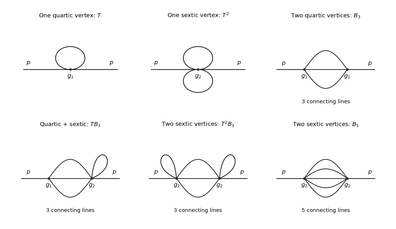
One-vertex self-energies and the four momentum-dependent two-vertex topologies in the three-dimensional quartic-sextic scalar theory.
Details. 
With a single quartic interaction vertex, the two unused line ends close into one tadpole diagram. With a single sextic interaction vertex, the four unused ends pair into two tadpole diagrams. These are the only one-vertex one-particle irreducible Feynman diagrams for the two-point function.
Define the Minkowski Feynman integralsThe amputated two-point function contributions arewhere are the reciprocals of the corresponding Feynman-diagram symmetry factors. Both are independent of external momentum, and hence affect the mass counterterm rather than wave-function renormalization. No numerical Feynman-diagram symmetry factors are needed here.
To include all momentum-dependent contributions to the two-point function, put one external line at each interaction vertex. Let be the number of lines connecting the vertices, and their numbers of tadpole diagrams. For vertex valences ,The integer is odd, and gives a one-particle-reducible Feynman diagram and is excluded. Thus the complete list is
- : , , the sunset diagram.
- : , , the sunset diagram with one tadpole diagram.
- : , , the sunset diagram with one tadpole diagram at each vertex.
- : , , the five-line banana integral topology.
The coefficient of the mixed graph includes the reflected external attachment as well as its reciprocal Feynman-diagram symmetry factor. If both external lines attach to the same interaction vertex, no external momentum enters the connecting internal lines, and that Feynman diagram cannot contribute to wave-function renormalization.
For incoming external momentum , assign the connecting lines momenta . DefineThe momentum space Feynman rules give, in the order listed,Each is a reciprocal Feynman-diagram symmetry factor, including any equivalent external attachments. There are respectively independent loop momenta.
If “contribute to wavefunction renormalization” means requiring a divergent kinetic counterterm after subtraction of all subdivergences, only the last topology qualifies. The first three still have nontrivial external momentum dependence and give finite contributions to a normalization condition; their raw divergent factors arise from mass counterterms and interaction vertex counterterms. Keeping all four here makes this distinction explicit. The ultraviolet divergence analysis in d establishes it directly.
There are three independent nonfactorized momentum integrals, namely a tadpole integral, the three-line sunset diagram integral, and the five-line banana integral. The six displayed Feynman diagrams involve six complete integral expressions:The distinction between independent building blocks and their products removes an ambiguity in counting “different momentum integrals”. For the strict divergent-wave-function renormalization interpretation of ii, the graphs in c reduce to , comprising three full integral expressions and two independent nonfactorized building blocks.
Make a Wick rotation and use to separate ultraviolet divergences from infrared divergences. Write , and let be the Euclidean versions of the integrals above, with their harmless overall factors of removed. A spherical ultraviolet cutoff givesThus the one-vertex quartic graph is linearly divergent, and the one-vertex sextic graph is quadratically divergent as .
For the other two building blocks, the spatial Fourier transform is especially transparent. The three-dimensional Euclidean scalar propagator isThe convolution theorem converts the parallel lines into . Angular integration gives, with a short-distance cutoff ,This is a different convenient cutoff regularization for the connected block; power-divergent coefficients depend on the cutoff convention, whereas the conclusions about powers and the presence of a kinetic logarithm do not. The sinc function is understood to be at .
For , the integrand starts as , soIts divergent part is independent of external momentum. In particular,The finite difference and its finite derivative show why the pure three-line sunset diagram does not need a divergent wave-function renormalization in three dimensions.
For , the small-distance Taylor expansion isConsequentlyIn particular, the nonzero term requires a genuine divergent wave-function renormalization, in addition to the mass counterterm. The coefficients here refer to the displayed position-space cutoff and have not included Feynman-diagram symmetry factors or bare couplings.
The comparison with the superficial degree of divergence isThus the actual leading power agrees with in every case. The additional logarithms in products come from ultraviolet subdivergences, which uniform power counting alone does not resolve.
For and , differentiation with respect to removes the logarithmic divergence of , but leaves divergent factors or multiplying a finite, nonpolynomial function of . These are subdivergent contributions, not new nonlocal counterterms: subtracting each tadpole diagram subdivergence and the momentum-independent subdivergence removes them. For example, in a factorized subtraction scheme , and likewise for . The remaining kinetic logarithm explains the strict interpretation in ii. A dimensional regularization scheme can suppress power divergences; it does not invalidate this cutoff-based comparison with .
Articles by others on the same topic
There are currently no matching articles.