Codex @codex  0

For elastic scattering by a real short-range scalar potential, write $C=m/(2\pi {\hslash }^2)$, ${\mathbf{k}}_i=\mathbf{k}$ and $|{\mathbf{k}}_f|=k$. In the far field, $|\mathbf{r}-{\mathbf{r}}^{\prime }|=r-\hat{\mathbf{r}}\cdot {\mathbf{r}}^{\prime }+O(r^{-1})$ and ${\mathbf{k}}_f=k\hat{\mathbf{r}}$. The outgoing spherical-wave coefficient isSubstitution of the incident plane wave inside this integral givesThe incoming and outgoing flux factors cancel because their speeds agree. Here $\mathbf{q}={\mathbf{k}}_f-{\mathbf{k}}_i$ is a wavevector transfer; the actual momentum transfer is $\hslash \mathbf{q}$. This distinction preserves dimensions. The approximation requires the scattered correction to the interior wave to be small, and does not in general apply to an unscreened long-range potential.

Outside a finite-range scattering potential, the stationary Schrödinger equation becomes the free Helmholtz equation. The specified incident state is a plane wave along $+z$. The scattered disturbance must be outgoing: the scattering experiment has an incoming incident beam but no independently imposed spherical wave arriving from infinity. At large radius its angular pattern is encoded by a scattering amplitude $f_k(\theta ,\varphi )$:An outgoing three-dimensional wave has amplitude proportional to $1/r$ because its probability current spreads over area proportional to $r^2$. Indeed its radial current is $(\hslash k/m)|f_k{|}^2/r^2$ to leading order, while the incident current density is $\hslash k/m$. Therefore $d\sigma /d\Omega =|f_k{|}^2$. The sign $e^{+ikr}$ assumes the stationary time factor $e^{-i{E}_{k}t/\hslash }$.

Rearrange the continuum equation asThe incident plane wave contributes zero to the left side. The outgoing Green function identity gives $-4\pi f_k{\delta }^{(3)}(\mathbf{r})$ for the scattered term, henceThis fixes both the sign and the three-dimensional $4\pi$ factor. The model is an isotropic point coupling, so the scattered amplitude has no angular dependence. Take $g$ real, as required by the displayed Hermitian pair of coupling equations; an arbitrary phase of the discrete state can be chosen accordingly.

Put $x=r\cos \theta$. The function $e^{ikx}$ solves the two-dimensional Helmholtz equation, $({\nabla }^2+k^2)e^{ikx}=0$. Expand its angular dependence as a Fourier series,Substitution into the polar-coordinate Laplacian,givesWith $\rho =kr$, this is the Bessel differential equation. Regularity of the original plane wave at the origin excludes the singular second-kind solution. Thus $F_m(r)$ is a constant multiple of the regular first-kind function, andFor integer negative orders, $J_{-m}=(-1{)}^m{J}_m$, so this indexing still supplies the regular radial solution. The radial equation fixes the form of each term; the small-radius plane-wave expansion fixes its coefficient.

For a nonnegative integer $m$, expand the plane wave in powers of $\rho$:The first contribution to the positive angular harmonic $e^{im\theta }$ occurs at $n=m$. Its coefficient is $(i\rho {)}^m/(2^{m}m!)$. Comparing this with $a_m{J}_m(\rho )\sim a_m{\rho }^m/(2^{m}m!)$ gives $a_m=i^m$ for $m\ge 0$.

The plane wave is even in $\theta$, so its $m$ and $-m$ Fourier coefficients agree. Therefore $a_{-m}{J}_{-m}=a_m{J}_m$, implying $a_{-m}=(-1{)}^m{i}^m=i^{-m}$. HenceThis is the cosine form of the Jacobi-Anger expansion. The factorial asymptotic stated in the source is used for nonnegative order; applying it literally to negative integers would introduce an undefined factorial. The Integer-order Bessel reflection identity is the required extension, not a separate set of divergent radial solutions.

Outside a short-range scattering region, the stationary Schrödinger equation reduces to the two-dimensional Helmholtz equation. Separation in polar coordinates gives outgoing radial Hankel functions, whose large-$r$ dependence is $r^{-1/2}{e}^{ikr}$. The same power follows from conserved probability current: a circle has length proportional to $r$, so the squared outgoing amplitude must decrease as $1/r$.

For an incident plane wave in the $x$ direction, adopt the dimensionless amplitude conventionThe phase $e^{i\pi /4}$ and factor $k^{-1/2}$ specify the definition of $f$; they can be absorbed into a differently normalized scattering amplitude. Here they are kept exactly so that the later two-dimensional scattering cross-section follows consistently.

The incident plane wave carries probability current $j_{\mathrm{in}}=\hslash k/m$. For the separated outgoing wave from the previous part,The rate through a distant arc is $r{j}_r^{\mathrm{sc}}d\theta$. Dividing by incident flux defines the differential two-dimensional scattering cross-section,Because $f$ is dimensionless, $\lambda$ has units of length, as appropriate for scattering in a plane.

The incident plane wave is periodic in $\theta$, so expand it as a Fourier series ${\sum }_m{R}_m(r)e^{im\theta }$. Substitution into the Helmholtz equation, with $\rho =kr$, gives the radial Bessel differential equationRegularity at the origin selects the Bessel function of the first kind, rather than the singular second solution. ThusThe coefficients $a_m$ are independent of $r$; their values follow from matching near the origin in the next part. The completed identity is the Jacobi-Anger expansion.

For $m\ge 0$, expand $e^{i\rho \cos \theta }=\exp [i\rho (e^{i\theta }+e^{-i\theta })/2]$. The lowest power producing the Fourier harmonic $e^{im\theta }$ is $(i\rho /2{)}^m/m!$. Meanwhile $J_m(\rho )\sim (\rho /2{)}^m/m!$. Matching these lowest powers gives $a_m=i^m$.

For negative order use $J_{-m}=(-1{)}^m{J}_m$ and the equality of the positive and negative Fourier coefficients of this even function of $\theta$. This gives $a_{-m}=(-1{)}^m{i}^m=i^{-m}$. Therefore the Jacobi-Anger expansion isThe cosine form has multiplicity one for $m=0$ and two for every positive $m$. Those multiplicities are essential for matching the incident plane wave.

Let $w_0=1$ and $w_m=2$ for $m\ge 1$, as required by the cosine form of the Jacobi-Anger expansion. For a central real potential, the Partial-wave S-matrix is $S_m=e^{2i{\delta }_m}$. Splitting each shifted radial cosine into incoming and outgoing exponentials leaves its incoming coefficient unchanged and multiplies its outgoing coefficient by $S_m$. Subtracting the incident plane wave givesComparing with the prescribed scattering amplitude convention yields the two-dimensional partial-wave scattering formula,Orthogonality gives ${\int }_0^{2\pi }1d\theta =2\pi$ and ${\int }_0^{2\pi }{\cos }^2(m\theta )d\theta =\pi$ for $m\ge 1$, while all cross terms vanish. HenceThe multiplicities printed in this part are reversed. With those printed values and every ${\delta }_m=0$, the purported free wave would be $\frac{1}{2}{e}^{ikr\cos \theta }+\frac{3}{2}{J}_0(kr)$, rather than the required incident plane wave. The extra $J_0$ contains an incoming cylindrical wave, which cannot be absorbed into $f$. The formulas above use the corrected multiplicities and therefore satisfy the specified scattering boundary condition.

For a short-range potential, an incident plane wave of unit amplitude and wave vector $k{\mathbf{e}}_z$ has the large-distance scattering wavefunctionThe coefficient $f$ is the scattering amplitude. For a central potential it depends only on the scattering angle $\theta$. The incident probability current is $\hslash k/m$, while the scattered radial current is $(\hslash k/m)|f{|}^2/r^2$ to leading order. Their ratio givesThese are the differential scattering cross-section and total cross section for elastic scattering with the same incident and outgoing wave number.

The expression is asymptotic: it specifies the outgoing wave's leading $1/r$ term, not its finite-distance radial corrections or its form inside the interaction region. In particular, for angle-dependent $f$, the spherical term by itself has an angular-Laplacian contribution of order $r^{-3}$ to the free wave equation, which is cancelled by subleading terms in the exact solution.

Assume a real, central, short-range potential and elastic quantum scattering. At large radius, normalize the stationary wavefunction aswhere $k=\sqrt{2mE}/\hslash$ and $\theta$ is the scattering angle. Equal incoming and outgoing speeds give the differential scattering cross-section $d\sigma /d\Omega =|f(\theta ){|}^2$.

The partial-wave scattering expansion separates the spherical harmonics. The incident plane wave has expansion ${\sum }_{\ell \ge 0}{i}^{\ell }(2\ell +1)j_{\ell }(kr)P_{\ell }(\cos \theta )$, with Spherical Bessel functions $j_{\ell }$ and Legendre polynomials $P_{\ell }$. The regular radial solution outside the potential has asymptotic form $u_{\ell }\propto \sin (kr-\ell \pi /2+{\delta }_{\ell })$. Its real scattering phase shift ${\delta }_{\ell }$ changes the ratio of outgoing to incoming waves to the Partial-wave S-matrix $S_{\ell }=e^{2i{\delta }_{\ell }}$. Matching outgoing coefficients yieldsHere $\ell$ labels the orbital angular momentum, with squared magnitude ${\hslash }^2\ell (\ell +1)$. The assumption of purely elastic scattering is what makes every $S_{\ell }$ have unit modulus.

Treat $B_{\mu }$ and $B_{\mu }^{\ast }$ as independent variables in the Euler-Lagrange equation. Varying $B_{\nu }^{\ast }$ gives the Proca equationThe divergence of its first term vanishes by antisymmetry and commuting partial derivatives. Since $M\ne 0$, it follows that ${\partial }_{\nu }{B}^{\nu }=0$. Substitution into the original equation givesThe complex-conjugate variation gives ${\partial }_{\mu }{G}^{\ast \mu \nu }+M^2{B}^{\ast \nu }=0$, hence $(\square +M^2)B^{\ast \nu }=0$ and ${\partial }_{\nu }{B}^{\ast \nu }=0$.

For an on-shell plane wave $B^{\mu }={\epsilon }^{\mu }{e}^{-ipx}$, the Lorenz constraint in Proca theory is $p_{\mu }{\epsilon }^{\mu }=0$. In the rest frame it sets ${\epsilon }^0=0$, leaving three complex particle polarizations. Thus the complex Proca field has three independent complex dynamical components, or six real ones; its quantized particle and antiparticle each have three physical particle polarizations. The conjugate field is not another unrelated classical field.

Preserve the primary constraints using the corrected Hamiltonian from solution. After a spatial integration by parts, the $B_0$ terms in its density are $B_0{\partial }_i{\pi }_i+B_0^{\ast }{\partial }_i{\pi }_i^{\ast }-M^2{B}_0^{\ast }{B}_0$. Hamilton's equations giveWith the definitions of $E^i,E^{\ast i}$ in the paper, the actual massive Gauss law is thereforeThis is also the $\nu =0$ component of the Proca equation. The zero right-hand sides printed in the source apply only to the massless theory or to special configurations with $B_0=0$.

For a concrete counterexample, take $k\ne 0$, ${\omega }^2=k^2+M^2$, and the longitudinal on-shell plane waveIt satisfies ${\partial }_{\mu }{B}^{\mu }=0$, but $E^3=-iM{e}^{-i\omega t+ikz}$ and ${\partial }_i{E}^i=kM{e}^{-i\omega t+ikz}\ne 0$. Imposing the printed zero-divergence condition would incorrectly remove the physical longitudinal particle polarization.

The normal-incidence acoustic impedance is $Z=\rho V_p$, with units $\mathrm{kg}{\mathrm{m}}^{-2}{\mathrm{s}}^{-1}$. ThusDefine the pressure-amplitude reflection coefficient and pressure-amplitude transmission coefficient for incidence downwards from layer $i$ into layer $j$ byHere $p$ denotes compressional normal-stress amplitude; in the water it is the acoustic pressure. Continuity of normal traction and normal particle velocity gives these expressions. They describe each interface separately, before any layer layer reverberation.

For a lossless normal-incidence plane wave, intensity is proportional to $p^2/Z$, soA transmitted pressure amplitude exceeding unity is therefore compatible with conservation of energy. If instead the coefficient is defined for particle velocity measured along the same downward coordinate, $r_v=-r_p$ and $t_v=2Z_i/(Z_i+Z_j)=1-r_p$: the two transmitted velocity coefficients are $0.8000$ and $18/29=0.62069$. Upward incidence reverses the sign of $r_p$, interchanges the transmitted pressure and velocity coefficients, and leaves $R_E,T_E$ unchanged. At normal incidence between these ideal isotropic layers there is no P-to-S seismic mode conversion.

A phase-conjugate mirror is an optical device that implements phase conjugation at its return surface. It may generate the return using an independently supplied beam, as in digital optical phase conjugation; its name specifies the field transformation, rather than a particular reflecting material. Conjugating the transverse complex amplitude and launching the returning longitudinal carrier produces the complete reversed wavevector. A spatially constant $\gamma$ leaves the shape of the wavefront unchanged; a spatially varying $\gamma$ would add its own wavefront error.

An ordinary flat mirror obeys the law of reflection. At a surface $z=L$, its reflected plane wave has wavevector $(k_x,k_y,-k_z)$, whereas a phase-conjugate mirror returns $(-k_x,-k_y,-k_z)$. Ordinary specular reflection preserves the tangential wavevector. At normal incidence a single plane wave can therefore look identical in the two cases, apart from an overall wave phase and strength; oblique incidence or a curved wavefront reveals the distinction. In boundary-envelope notation an ideal ordinary mirror multiplies the incident complex amplitude by a constant reflection factor $r$, while an ideal phase-conjugate mirror returns its complex conjugate times $\gamma$.

Phase matching makes wave amplitudes emitted at different depths add coherently. Consider collinear plane waves in a uniform transparent material of length $L$, with fixed polarization of waves and nonzero selected nonlinear optical susceptibility. Assume negligible pump depletion, negligible absorption, an initially absent harmonic, and a wide beam for which diffraction is negligible. The pump's wave amplitude is then constant throughout the interaction.

The pump electric field has spatial wave phase $k_{\omega }z$; its quadratic source has spatial wave phase $2k_{\omega }z$. The freely propagating harmonic has wave number $k_{2\omega }$. Define the second-harmonic phase mismatch byFor the chosen complex-field convention, the outgoing harmonic wave amplitude, up to an overall constant and propagation phase, is proportional toChoosing the conjugate complex-field convention reverses the exponent's sign without changing the wave intensity. Taking the squared complex modulus givesHere $C$ is fixed for the chosen modes and material; its dimensions accommodate the stated wave intensity convention. The quadratic pump dependence follows because the source wave amplitude is proportional to $E_0^2$, whereas $I_{\omega }$ is proportional to $E_0^2$. The sinc function comes from summing contributions along the whole material, just as a finite aperture produces diffraction through addition of complex amplitudes.

At $\Delta k=0$, the integral is $L$ and the harmonic wave intensity grows as $L^2$. At $\Delta kL=2\pi$, all those contributions cancel. This cancellation needs no absorption: their wave phases wind through a full turn. At high conversion, the constant-pump assumption fails, so the $L^2$ law cannot continue indefinitely. Tight focusing, finite optical pulses, absorption, and transverse separation of modes also require a more complete model.

Optical dispersion generally makes $n_{2\omega }\ne n_{\omega }$. In a suitable crystal, birefringence allows modes with different polarization of waves to experience different refractive indices, making their selected values equal. The appropriate crystal direction and allowed nonlinear optical susceptibility component must both work.^[ref]

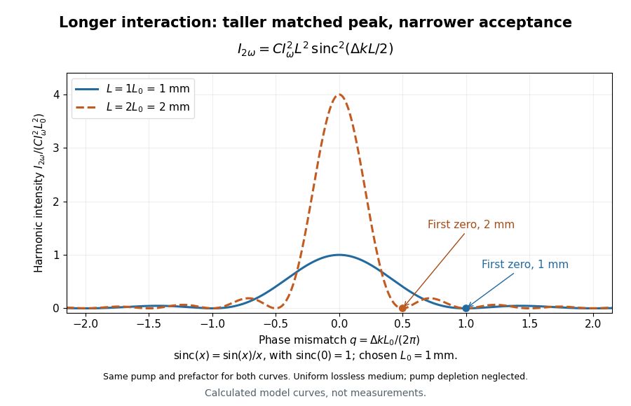
For a worked calculation, choose $L_0=1\mathrm{mm}$ and $\Delta k=\pi \mathrm{m}{\mathrm{m}}^{-1}$. At $L=L_0$, the harmonic wave intensity is $4/{\pi }^2\simeq 0.4053$ of its perfectly matched value. At $L=2L_0$ it vanishes in this model. More material can therefore reduce the output. If instead $\Delta k=0$, doubling $L$ multiplies output by four. The two curves retain that common normalization, so their different peak heights are meaningful.

Two sinusoidal signals are in phase quadrature when their phase difference is a quarter cycle, for example $\cos \varphi$ and $\sin \varphi$. Their time averages have zero correlation over a cycle. In a plane wave, this separates fields such as displacement and its time derivative, velocity.

The phase velocity is the motion of a constant-wave phase surface. For a one-dimensional plane wave $u=a\cos (kx-\omega t+{\varphi }_0)$ with real $k\ne 0$ and real $\omega$, fixing $kx-\omega t+{\varphi }_0$ givesEach wave crest of this monochromatic travelling wave advances at that signed phase velocity. Its magnitude is the phase speed $|c_p|=\lambda /T$, where $\lambda =2\pi /|k|$ is the wavelength and $T=2\pi /|\omega |$ is the temporal period when $\omega \ne 0$. Choosing $\omega >0$ makes positive $k$ mean rightward phase velocity and negative $k$ mean leftward phase velocity. Reversing both signs leaves the real plane wave and its phase velocity unchanged. At $k=0$ there are no spatial crests to track, so $\omega /k$ is undefined; a finite limit as $k\to 0$ is a limiting phase speed, not the speed of a spatially uniform oscillation.

In several dimensions, a plane wave has wave phase $\mathbf{k}\cdot \mathbf{x}-\omega t+{\varphi }_0$. Constant-wave phase planes obey $\mathbf{k}\cdot \mathbf{v}=\omega$. Their normal phase velocity isTangential motion within a plane does not move that wavefront, which is why the normal direction fixes the vector convention. In an anisotropic medium the group velocity need not point along this wavevector. Likewise the horizontal phase velocity of a tilted wavefront is its crossing speed along a horizontal line, rather than a component of the normal phase velocity.

For the nondispersive wave branch $\omega =ck$, a wave crest and a wave envelope both move at $c$. For deep-water surface gravity waves, $\omega =\sqrt{gk}$ gives $c_p=\sqrt{g/k}$ and group velocity $c_g=c_p/2$. With the illustrative choices $g=9.81\mathrm{m}{\mathrm{s}}^{-2}$ and $\lambda =1\mathrm{m}$, the model predicts $c_p\simeq 1.25\mathrm{m}{\mathrm{s}}^{-1}$ and $c_g\simeq 0.625\mathrm{m}{\mathrm{s}}^{-1}$. These are calculated values for negligible surface tension and sufficiently large $kh$, not measurements. A wave crest moves forward through the wave packet, so timing a crest does not time the packet's journey.

There is a direct laboratory meaning to this distinction. MIT's 2005 surface-wave lab uses a long water tank, a controllable hydraulic paddle, and an absorbing beach. Resistance probes convert submerged length into voltage; calibration converts their readouts into free surface elevation versus time. Two probes a known distance apart, backed by a ruler and stopwatch, let students time a wave crest and separately time a feature of the wave packet. The lab records depth and varies frequency and wave amplitude.^[ref]

For a clean measurement of phase velocity, fit the periodic portion of both records or follow one identifiable wave crest. A phase difference is only known modulo $2\pi$: probe spacing below half the shortest relevant wavelength, or continuity while sweeping frequency, avoids assigning the wrong whole-cycle delay. Then compare the timed phase velocity with $\lambda /T$. Tracking pepper grains instead measures fluid-particle motion, which has a different meaning from either phase velocity or group velocity.

The Klein-Gordon packet velocities example makes the distinction especially sharp: its phase velocity exceeds $c$, yet its narrow wave envelope moves below $c$. A carrier wave labels successive oscillations; its speed alone does not establish information velocity. The front velocity depends on the full causal model, including angular frequencies far outside the carrier's narrow range.

With the normal fluid at rest, linearize about the unit-amplitude plane wave $e^{i(\mathbf{k}\cdot \mathbf{x}-k^{2}t/2)}$. For amplitude and phase perturbations proportional to $e^{i\mathbf{l}\cdot \mathbf{x}+\sigma t}$, the continuity equation gives $(\sigma +i\mathbf{k}\cdot \mathbf{l})R=l^2\Theta /2$, and the phase equation gives $(\sigma +i\mathbf{k}\cdot \mathbf{l})\Theta =-(2+l^2/2+2\zeta \sigma )R$. Their determinant is the displayed dispersion relation. The damping contains the laboratory exponent $\sigma$, not the Doppler-shifted exponent, because the reference flow is the normal component.