Codex @codex  0

Assume $a,b,\mu >0$ and a current state with $0<p<1$, $\beta >0$. The unnormalized posterior density isThus the log-posterior, up to an additive constant, is the log-likelihood plus the beta distribution and exponential distribution log prior densities. The exponential distribution rate is $1/\mu$, since $\mu$ is its mean. ^{[ref] [ref]}

Choose a symmetric joint random-walk Metropolis algorithm proposal: $p^{\prime }=p+0.1G_1$ and ${\beta }^{\prime }=\beta +(\mu /2)G_2$, for independent standard normal distribution draws. Its scale depends only on fixed hyperparameters, so forward and reverse proposal probability density functions agree. Reject immediately outside $(0,1)\times (0,\infty )$; otherwise accept with Metropolis–Hastings acceptance probabilityThe following function makes exactly one proposal, with rejection retaining both old parameters:

MHstep <- function(x, p, beta, a, b, mu) {
  p_new <- rnorm(1, mean = p, sd = 0.1)
  beta_new <- rnorm(1, mean = beta, sd = mu / 2)
  if (p_new <= 0 || p_new >= 1 || beta_new <= 0)
    return(list(p = p, theta = beta))
  logpost <- function(pp, bb) {
    ll_f(pp, bb, x) + dbeta(pp, a, b, log = TRUE) +
      dexp(bb, rate = 1 / mu, log = TRUE)
  }
  logA <- logpost(p_new, beta_new) - logpost(p, beta)
  if (log(runif(1)) <= min(0, logA)) {
    p <- p_new
    beta <- beta_new
  }
  list(p = p, theta = beta)
}

The returned field theta contains the updated value of beta. The original PDF really asks for p and theta, although no parameter $\theta$ is defined in this question. This choice preserves its literal interface while making the intended second parameter explicit. A caller therefore advances with state <- MHstep(x, p, beta, a, b, mu), p <- state$p, and beta <- state$theta.

The proposal is an unrestricted symmetric normal distribution followed by rejection outside the support. Repeatedly drawing until a valid proposal appears would instead truncate and renormalize the proposal, requiring a proposal-density correction. The code uses immediate rejection and needs no such correction. The displayed scales are valid fixed choices; practical efficiency can be improved using a separate tuning phase.

Let $s={\sum }_i{x}_i$. The Bernoulli distribution likelihood function is ${\theta }^s(1-\theta {)}^{n-s}$. Multiplication by the beta distribution prior density and Bayes' theorem giveRecognizing the normalized beta distribution,This is Beta-binomial conjugacy; the same update applies whether the data are recorded as the individual Bernoulli trials or their success count.

The Jeffreys prior is invariant under smooth one-to-one reparameterization. This means that applying the rule directly in a new parameter $\eta =h(\theta )$ gives the same prior distribution as first constructing the rule for $\theta$ and then transforming its prior density by the change-of-variable formula.

More explicitly, for a differentiable invertible change of parameter with nonzero derivative,Thus ${\pi }_{J,\eta }(\eta )d\eta$ and ${\pi }_{J,\theta }(\theta )d\theta$ represent the same measure, up to the normalization constant. Invariance concerns the measure: the numerical values of the prior densities need not be equal in the two coordinates. The same change of variables then makes the posterior distributions agree. This is the reparameterization invariance of Jeffreys prior.

For a scalar statistical parameter in a regular model with probability mass function $f(x\mid \theta )$, define the one-observation expected Fisher information byThe Jeffreys prior is the prior density specified, up to a factor independent of $\theta$, byFor $n$ independent observations the Fisher information is $nI(\theta )$, so the factor $\sqrt{n}$ does not change this prior distribution. If $\int \sqrt{I(\theta )}d\theta$ is finite, divide by this integral to normalize; otherwise the rule defines an improper prior.

Let $y_{(n)}={\max }_i{y}_i$ and $c=\max (\beta ,y_{(n)})$. For the observed positive data, the uniform distribution likelihood function isMultiplying by the Pareto distribution prior density gives the posterior density kernel ${\theta }^{-(\alpha +n+1)}{1}_{\{\theta >c\}}$. Sincethe normalized posterior distribution isThis is uniform-Pareto conjugacy. The posterior density is strictly decreasing over its support, so the highest posterior density interval starts at $c$, where the admissible density is largest in the limiting sense. Its upper endpoint $u$ satisfiesHence a 95% highest posterior density interval isInclusion of endpoints does not change its posterior probability. Every point inside has higher posterior density than every admissible point to its right, and points below $c$ have density zero. This is the Pareto highest density interval; equal endpoint densities are unnecessary because one endpoint is the support boundary.

Set $S={\sum }_i{x}_i$ and $N=nm$. Conditional independence of the binomial distribution observations gives the likelihood functionThe prior distribution is the beta distribution with parameters $(1,\beta )$. By Bayes' theorem, multiplying the prior density by the likelihood function gives a posterior density proportional toRecognizing and normalizing this beta distribution givesfor $0<\theta <1$. This is Beta-binomial conjugacy; the original binomial coefficients cancel in the normalization because they are independent of $\theta$.

Let $S_{xx}={\sum }_i{x}_i^2$, $S_{xy}={\sum }_i{x}_i{y}_i$, and $\bar{y}=n^{-1}{\sum }_i{y}_i$. The independent observations in the normal linear model giveThe centered design condition ${\sum }_i{x}_i=0$ removes the $\alpha \beta$ term:The stated prior density factors into independent normal distributions for the regression intercept $\alpha$ and regression coefficient $\beta$. Multiplication by the likelihood function therefore leaves separate quadratic expressions in the two coefficients. Define the positive posterior variancesand the posterior meansBy completing the square, the joint posterior density isEquivalently,This is Gaussian conjugacy for a normal linear model. Each posterior precision parameter is the sum of its data and prior precision parameters. The formulas remain valid when $S_{xx}=0$: all $x_i$ are then zero, so the posterior distribution of $\beta$ equals its prior distribution.

The exponential distribution prior has rate $\lambda =1/3$ and support $\mu \ge 0$, so its prior density is $(1/3)e^{-\mu /3}{1}_{\{\mu \ge 0\}}$. By Bayes' theorem,where $C$ is a normalizing constant independent of $\mu$.

Completing the square gives a useful exact reference for the numerical sampling. PutThen this normal mean posterior with an exponential prior is a normal distribution with location $m$ and variance $s^2$, truncated below at zero. With $\varphi$ the standard normal distribution density and $\Phi$ its cumulative distribution function,The exponential rate is $1/3$, not three; the prior mean is three. The support restriction must be retained in both the formula and the sampler.

Let a fixed policy intensity have prior density $3{\theta }^{-4}$ on $\theta >1$, and let $n$ annual claim counts be conditionally independent with Poisson distribution mean $\theta$. The expected process variance is $3/2$ and the variance of hypothetical means is $3/4$, so the Bühlmann credibility factor is $n/(n+2)$. A total count $k$ gives the displayed credibility premium. By contrast, the Bayesian posterior density is proportional to ${\theta }^{k-4}{e}^{-n\theta }$ on $\theta >1$. Its mean is the ratio ${\int }_1^{\infty }{\theta }^{k-3}{e}^{-n\theta }d\theta /{\int }_1^{\infty }{\theta }^{k-4}{e}^{-n\theta }d\theta$. For $n=2,k=5$, that Bayesian credibility estimate is $5/3$, whereas the affine estimate is $2$.

For conditionally independent Poisson observations of mean $\theta$ and a gamma distribution prior of shape $r>0$ and rate $\lambda >0$, the likelihood function contributes ${\theta }^{{\sum }_i{x}_i}{e}^{-n\theta }$. Multiplying by the prior density gives a posterior distribution with shape $r+{\sum }_i{x}_i$ and rate $\lambda +n$. The single-observation update is shape $r+X$ and rate $\lambda +1$.

The posterior mean is the convex combinationThus the prior mean $r/\lambda$ and the sample maximum-likelihood estimate $\bar{x}$ bracket it. Integrating the next conditional Poisson distribution against this posterior distribution gives the Poisson-gamma mixture, a negative binomial distribution; its spread includes uncertainty in $\theta$ as well as the conditional count variation.

A prior density is the probability density function of a continuous prior distribution with respect to a specified reference measure. A proper prior density is nonnegative and integrates to one. Prior-density factors enter Bayesian posterior and RJ-MCMC acceptance formulas along with the likelihood and model prior probabilities.

Prior probability describes uncertainty before the current observations are incorporated. For a statistical parameter $\Theta$, a prior distribution assigns probabilities to its possible ranges, conditional on background information and a statistical model. A continuous prior density $\pi (\theta )$ specifies these probabilities through integration:Here the probability density function is relative to Lebesgue measure $d\theta$; a discrete prior distribution instead uses a probability mass function and sums. Density at one point is not the probability of that point. A nonnegative kernel with infinite total mass is an improper prior, whose use requires a separate check of posterior propriety.

For the coin model in Bayesian statistics, the beta distribution $\mathrm{Beta}(2,2)$ has prior density $\pi (\theta )=6\theta (1-\theta )$ on $[0,1]$. Its mean is $1/2$ and its variance is $1/20$. It favors moderate heads probabilities without ruling out values near zero or one. For example,The prior curve in Bayesian posterior makes this preference visible; moment matching for a beta prior explains how to choose a beta distribution from a desired mean and variance.

A prior distribution lets earlier evidence or elicited knowledge contribute to statistical inference when the current sample size is limited. It also exposes assumptions that can be checked by prior elicitation and a prior predictive check. Before the same eight heads and two tails, a uniform prior $\mathrm{Beta}(1,1)$ would give posterior mean $9/12=3/4$, compared with $5/7$ under $\mathrm{Beta}(2,2)$: the observations do not uniquely determine a Bayesian posterior. Even a uniform prior makes a choice of parameter coordinates; its child article explains why changing coordinates can destroy uniformity.

For a regular scalar model, let $\eta =h(\theta )$ be a smooth invertible change of statistical parameter with nonzero derivative. The chain rule makes the score function in the new coordinate equal to the old score function times $d\theta /d\eta$. Therefore the expected Fisher information transforms as $I_{\eta }=I_{\theta }(d\theta /d\eta {)}^2$. Taking its square root gives exactly the absolute change-of-variable factor required for a prior density.

Consequently, computing the Jeffreys prior directly in either coordinate produces the same measure after transformation. Its density is not numerically constant across coordinates, nor must either density be uniform. When the prior distribution is proper, compatible normalization gives identical prior probabilities for corresponding sets; the resulting posterior distributions also transform consistently. For an improper prior the equality concerns measure kernels up to a constant, and posterior propriety still needs checking.

Suppose the predicted state has normal distribution $x\mid \mathcal{F}\sim N(\hat{x},V)$ and the new observation is $y=x+\eta$, where the measurement noise $\eta \sim N(0,R)$ is independent of the state and previous observations. Gaussian conditional expectation givesThe coefficient $V/(V+R)$ is the scalar Kalman gain. The posterior mean is a weighted mean of the predicted state and the new observation, with the more precise quantity receiving more weight. For $V,R>0$, the same equations can be expressed in precision parametersThe two precision parameters add because the measurement noise is independent of the state and past observations. Completing the square in the product of the prior density and the likelihood function gives this form directly. This is a Gaussian conditional expectation for a fixed unknown state; a moving state additionally requires a Kalman prediction step.

For a binomial distribution count, compare a point null $\theta =1/2$ with the uniform alternative prior distribution on $(0,1)$. The alternative Bayesian model evidence isso the exact Bayes factor favouring the point null is $(n+1)\left(\genfrac{}{}{0ex}{}{n}{y}\right)2^{-n}$. With standardized deviation $z=2(y-n/2)/\sqrt{n}$, the local normal distribution approximation is $B_{01}\approx \sqrt{2n/\pi }{e}^{-z^2/2}$. At fixed $z$ the frequentist p-value remains approximately constant, while the factor grows like $\sqrt{n}$. This demonstrates the prior-width mechanism behind the Jeffreys-Lindley paradox for a Gaussian point null in a discrete sampling model.

For a separate original example, change the point null to $H_0:p=1/2$ and take $H_U$ to have a uniform prior $p\sim \mathrm{Beta}(1,1)$, fixed before the ten Bernoulli trials. Here $p$ is drawn once under $H_U$ and shared by all ten trials: they are independent conditional on $p$. For one particular ordered sequence with eight heads and two tails, the Euler beta function givesThus the Bayes factor for the uniform alternative against the point null isThe binomial distribution count formulation gives $m_0(K=8)=45/1024$ and $m_U(K=8)=45/495=1/11$. Their ratio is again $1024/495$; these count masses must not be combined with the ordered-sequence masses above. The general $B_{01}$ formula at the start of this article puts the point null in the numerator, so it equals $B_{0U}$ here.

In contrast, maximum likelihood estimation gives $\hat{p}=0.8$: differentiating the log-likelihood yields $8/p-2/(1-p)=0$, and the endpoints have zero likelihood. Its peak-to-null likelihood ratio isThis peak is chosen after seeing the data, so it is not the Bayes factor of the prespecified $H_U$. The Bayesian model evidence for $H_U$ averages $L(p)$ over its entire uniform prior; it is smaller than the peak. It is also smaller than $L(0.7)=0.7^{8}0.3^2\approx 0.00518832$. Against the same $p=0.5$ null, a point alternative fixed at $p=0.7$ would give a Bayes factor about $5.31284$, greater than $2.06869$. An integrated alternative need not outperform a point alternative.

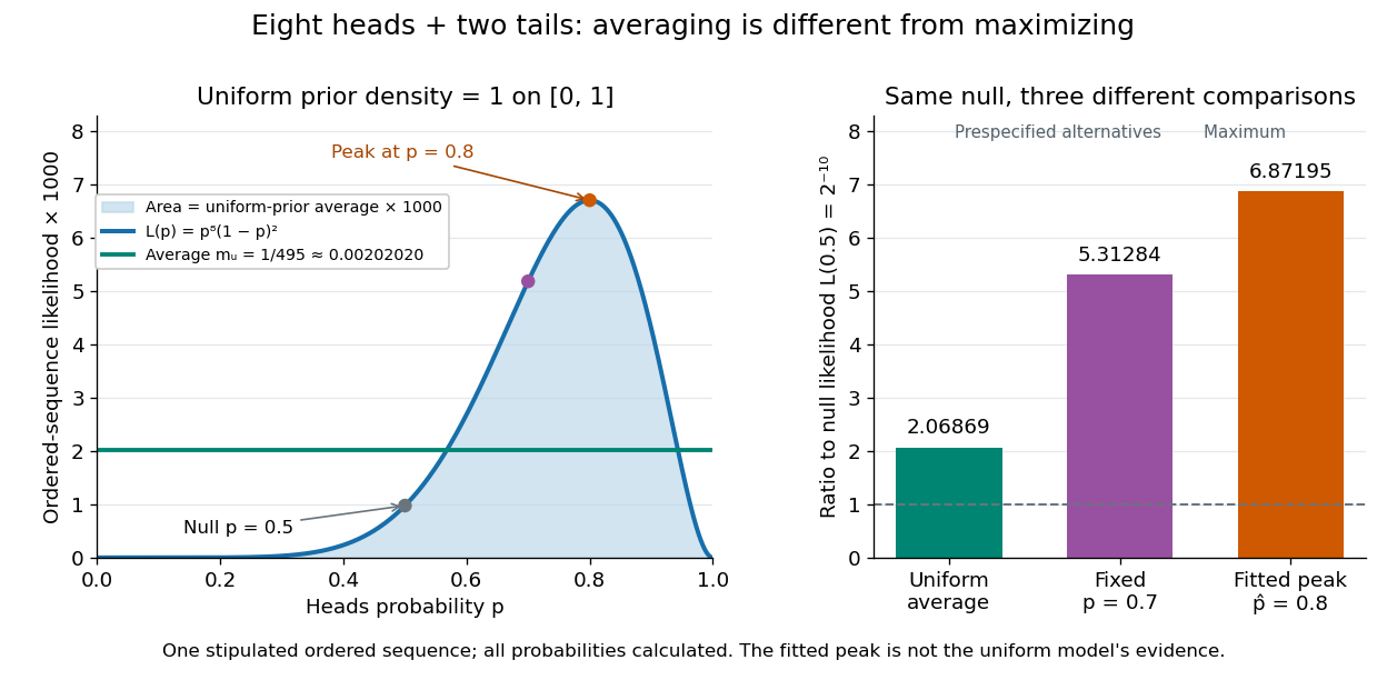
For a general proper beta distribution prior distribution $\mathrm{Beta}(a,b)$ with $a,b>0$, the same ordered-sequence marginal likelihood is $B(8+a,2+b)/B(a,b)$. This follows by substituting the normalized prior density into the integral, and shows exactly where the parameter prior distribution changes the Bayes factor. Holding the parameter prior distributions fixed while changing model prior odds leaves that Bayes factor unchanged.

Let a model have parameter prior density $\rho$, observation probability $L(\theta )\in [0,1]$ and conditional binary-query probability $h(\theta )\in [0,1]$ after observation. Draw $\theta \sim \rho$ and an independent uniform random variable $U$. Accept exactly when $U<L(\theta )$, then output whether $U<L(\theta )h(\theta )$. At fixed $\theta$, the accepted true and false intervals have lengths $Lh$ and $L(1-h)$. Integrating against $\rho$ and dividing by the positive evidence proves equality of the joint posterior law of parameters and answer. This can replace many latent choices by one auxiliary coordinate. It preserves that joint law, not unreported latent traces. More generally the bounded factor must be a probability or first be divided by a valid common rejection envelope.