Codex @codex  0

Let $s={\sigma }^2$ and $\vartheta =(s,{\tau }_1,\dots ,{\tau }_m)$. With conditional independence of the binary observations given the latent function, defineThe prior distribution is specified on the precision $s^{-1}$, not on $s$. Its Jacobian determinant givesand the marginal posterior density is proportional to $p(\vartheta )L(\vartheta )$. Working instead with precision or logarithmic coordinates is possible, provided all corresponding Jacobian determinants are included.

Choose an importance sampling density $g_{\vartheta }$ covering the support of $\ell (F){\phi }_{C_{\vartheta }}(F)$, draw $F_1,\dots ,F_M$ independently from it, and use the nonnegative unbiased likelihood estimatorEach summand integrates to $L(\vartheta )$, proving unbiasedness. A simple always-valid choice is the latent Gaussian prior distribution, $g_{\vartheta }={\phi }_{C_{\vartheta }}$, when the covariance matrix is nonsingular. Then the estimator is just the average of the bounded values $\ell (F_j)\in (0,1)$. For duplicate inputs, sample only the distinct latent values and multiply all likelihood contributions at each common input. A Gaussian approximation to the latent posterior distribution, or its mixture with the Gaussian prior distribution, can reduce relative variance while keeping complete support. Its approximation does not replace the exact weights.

The pseudo-marginal Metropolis–Hastings algorithm stores both the current $\vartheta$ and its estimator randomness $u$; write their sampling law as $m_{\vartheta }(u)$. Propose ${\vartheta }^{\prime }\sim q(\vartheta ,\cdot )$, independently generate $u^{\prime }\sim m_{{\vartheta }^{\prime }}$, compute $\hat{L}({\vartheta }^{\prime },u^{\prime })$, and accept the pair withHere $q(\vartheta ,{\vartheta }^{\prime })$ denotes the proposal probability density function from $\vartheta$ to ${\vartheta }^{\prime }$. On rejection retain both the old parameter and the old likelihood estimate. Initialize with a positive estimate. One must not independently refresh the denominator after rejection.

Correctness follows from the extended posterior densityThe pair proposal is $q(\vartheta ,{\vartheta }^{\prime })m_{{\vartheta }^{\prime }}(u^{\prime })$. Its Metropolis–Hastings acceptance probability simplifies to the displayed ratio, since the auxiliary densities cancel. Hence detailed balance holds for $\tilde{\pi }$. Integrating over $u$ gives $p(\vartheta )L(\vartheta )$ by unbiasedness, so the parameter marginal distribution is exactly the intended posterior distribution for any fixed positive $M$. This is exactness of the stationary target, not independent exact samples or a guarantee of rapid convergence. Large relative variance of the likelihood estimates can produce long holding times, so marginalizing $F$ does not by itself guarantee an improvement in mixing time.

Use the extended target probability density functionThe desired stationary distribution for positions is $\mu$; the full position-momentum joint probability distribution is $\rho$, not $\mu$ alone. Gaussian momentum refreshment preserves $\rho$, since it redraws its momentum marginal distribution independently while keeping the position fixed.

Let $R(x,p)=(x,-p)$ and $T=T_{\epsilon ,L}$ be the surrogate leapfrog integration map. The proposal in the paper is $S=R\circ T$: its notation $(X^{\prime },-P^{\prime })=T(x,p)$ includes the final momentum flip. Reversibility gives $RTR=T^{-1}$, so $S^2=I$. Both $R$ and $T$ preserve volume. Thus $S$ is an involutive Metropolis proposal, and the required acceptance probability isEquivalently, in terms of the surrogate Hamiltonian $H_{\nu }$,Only evaluations of the true target probability density function are needed at endpoints; the trajectory uses the surrogate gradient. Target and surrogate normalizing constants cancel.

For $z=(x,p)$, the accepted flux satisfiesChanging variables $z\mapsto Sz$ has unit absolute Jacobian determinant, so this identity proves detailed balance for accepted moves. The rejection mass stays at the same point and is also reversible. The accept/reject step therefore preserves $\rho$. Since momentum refreshment also preserves $\rho$, their composition and either phase of the alternating process preserve $\rho$. Projecting onto positions proves the position stationary distribution is exactly the original target. Stationarity alone does not establish uniqueness or convergence from every start; those require additional irreducible Markov chain and aperiodic Markov chain hypotheses.

There is a genuine defect in the printed smoothing claim. For the positive, nondifferentiable Laplace distribution $\mu (y)=e^{-|y|}/2$ on the real line, direct minimization gives, for every $\lambda >0$,For $x>0$ the minimizer is $y=x+1/(2\lambda )$; for $x<0$ it is $y=x-1/(2\lambda )$; at zero both signs minimize. Hence normalization leaves $\nu =\mu$, still nondifferentiable at zero. The displayed construction does not in general produce the asserted smooth surrogate. For example, the also nondifferentiable target $\mu (y)\propto e^{-y^4-|y|}$ makes that infimum $-\infty$ for every $x$, since the negative quartic term dominates the quadratic penalty. The invariance proof above is valid conditional on actually having a usable smooth surrogate, as the subsequent algorithm assumes.

A corrected sufficient construction is Moreau smoothing of a negative log-density. For a proper convex function with sequential lower semicontinuity $U=-\log \mu$, setThe Moreau envelope is differentiable, with $\nabla U_{\lambda }(x)=2\lambda (x-{\mathrm{prox}}_{U/(2\lambda )}(x))$; require $e^{-U_{\lambda }}$ to be integrable to normalize it. The signs differ from the printed formula. For the Laplace distribution, this givesa genuinely differentiable potential with integrable exponential tails. Using that surrogate with the boxed acceptance probability still targets the original Laplace distribution.

For this stellar population, let $m=M/M_{\odot }$ denote initial mass in units of the solar mass, and let $\tau =t/\mathrm{Gyr}$ denote present stellar age. Constant formation of equal numbers of stars per unit time makes the stellar age a uniform distribution on $[0,10]$ Gyr, so $Y=\tau /10$ is uniform on $[0,1]$. The normalized initial mass function has probability density function $f(m)=0.1m^{-2}$ for $m>0.1$, since ${\int }_{0.1}^{\infty }{m}^{-2}dm=10$. ConsequentlyThese formulae have the stated age and mass domains; outside them the relevant cumulative fractions saturate at zero or one. The probability integral transform makes $X$ uniform on $[0,1]$: $m=0.1/X$ gives $f(m)|dm/dX|=1$. The time-independent initial mass function and constant number formation rate give independence of $X$ and $Y$. All fractions here count objects, including white dwarfs, using the stipulated stellar evolution law.

A red giant hasThus the mass boundaries are $m=9/\tau$ and $m=10/\tau$ for positive $\tau$. Equivalently, for $0.9<m<1$ the red giant region runs from $9/m$ to the age cap $10$, and for $m\ge 1$ it runs from $9/m$ to $10/m$. There are no red giants with $m\le 0.9$. Boundaries have zero probability and their endpoint convention does not affect the fractions. In the uniform $(X,Y)$ square the red giant region is $9X<Y<10X$, with triangle vertices $(0,0)$, $(1/10,1)$ and $(1/9,1)$. The white dwarf region is the triangle $0<X<Y/10$.

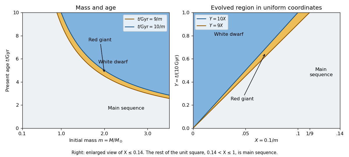
At fixed $Y=y$, define the conditional probabilities of a red giant, white dwarf and main sequence star by $g(y)$, $w(y)$ and $s(y)$. Their interval widths areIntegration over the uniform distribution of age gives the individual-star fractionsThe systems form a coeval binary population: the two binary star components have the same age. Their masses are independent, so $(X_1,X_2,Y)$ has uniform probability density function on $[0,1{]}^3$ and their states have conditional independence given $Y$. Unconditional independence of their states would be incorrect: older systems make both evolved states more likely. The law of total probability now givesThe subtraction removes the double counting of systems containing two red giants.

For $x>0$, $N(x)=\lfloor 1/x\rfloor$ and $T(x)=1/x-\lfloor 1/x\rfloor$. Iterating this Gauss continued-fraction map on an irrational number never reaches zero, and its continued fraction isThe branches $T:(1/(n+1),1/n)\to (0,1)$ have inverse $x_n(y)=1/(n+y)$, for $n\ge 1$. The change of variables formula for a probability density function gives, almost everywhere,The endpoints of these branches are a countable set of probability zero. Thus $T(X)$ and $X$ have the same distribution; this Gauss measure is an invariant measure for the Gauss continued-fraction map.

For $i\ne s$, the Markov property and the definition of transition intensity giveSumming over the possible pre-jump states gives the density of the expected Markov-chain entry count:For a finite-state continuous-time Markov chain, the chance of two or more jumps in this short interval is $o(du)$. There is no $q_{ss}$ contribution: diagonal entries of the infinitesimal generator encode exit rates, not jumps into the same state. With repeated entries possible, this density is an expected event rate rather than the probability density function of a single normalized random time.

For $1\le k\le n$, the nearest neighbour distance ${\rho }_{(k)}(x)$ is the $k$th order statistic of $D_i=|X_i-x|$. Each $D_i$ has continuous distribution function $p_x(r)$ on $[0,\infty )$. The probability integral transform makes $U_i=p_x(D_i)$ independent and identically distributed random variables with the uniform distribution on $(0,1)$. Monotonicity of $p_x$ gives $P=U_{(k)}$, a uniform order statistic. Strict monotonicity is not needed at this stage.

For $0<s<1$, counting observations below $s$ givesDifferentiating and cancelling consecutive terms gives the Beta distribution:The Gamma function identity $\Gamma (j)=(j-1)!$ identifies this with the stated normalization. Ratios of Beta function integrals yield the momentsThis is the probability content of a nearest neighbour ball identity, specialized to intervals on the real line.

Now write $f_0=f(x)>0$. The Lipschitz bound givesThusStrict positivity of the probability density function makes $p_x$ continuous and strictly increasing from zero to one, so its inverse function is defined for every $s\in (0,1)$.

For the requested conditional calculation, suppose $f_0^2\ge L$. At $r_0=s/f_0$ the preceding bound givesTherefore $r=p_x^{-1}(s)\le s/f_0$, and substituting in the approximation proves the inverse probability content bound for a Lipschitz density:The same argument works, without $f_0^2\ge L$, on the meaningful local range $0<s<1$ with $s\le f_0^2/L$.

Since the nearest neighbour density estimator obeys $f(x)/{\hat{f}}_{(k)}(x)=2(n+1)f_0{p}_x^{-1}(P)/k$, its conditional bound follows from the Beta distribution moments:Hence, under the printed location condition,The conditional inverse function bound also bounds $p_x^{-1}(P)$, so the expected value in this calculation is finite under those formal hypotheses.

There is, however, a genuine flaw in the original PDF: the printed condition $f(x)\ge \sqrt{L}$ has no admissible points when $f$ is strictly positive on all of $\mathbb{R}$. A probability density function on all of $\mathbb{R}$ cannot have Lipschitz constant zero, so $L>0$. Its Lipschitz bound forcesIntegrating this triangular lower envelope gives the Lipschitz density height boundThe inequality is strict because the probability density function has positive mass outside the finite interval. Thus $f(x)<\sqrt{L}$ everywhere. The last two conditional conclusions above are valid implications but vacuous as printed. Dropping strict positivity gives only $f(x)\le \sqrt{L}$, with equality forcing the entire probability density function to be the normalized triangular envelope. The local inverse bound does not justify replacing the printed condition by its reverse in the final expected value bound, since $P$ ranges over all of $(0,1)$.

For independent and identically distributed random variables with distribution function $F$, let $M_n={\max }_{1\le i\le n}{X}_i$ be the sample maximum. In extreme value theory, $F$ belongs to the maximum domain of attraction $D(G)$ of a nondegenerate distribution function $G$ when there exist $a_n>0$ and $b_n\in \mathbb{R}$ such thatat every continuity point of $G$. Thus the normalized sample maxima have convergence in distribution to $G$.

A positive measurable function $q$ has regular variation at infinity with index $\rho$, written $q\in {\mathrm{RV}}_{\rho }$, ifThe case $\rho =0$ defines a slowly varying function; equivalently a regularly varying function is $q(t)=t^{\rho }\ell (t)$ with $\ell$ a slowly varying function.

Write $\overline{F}=1-F$ for the survival function and $x_F=\sup \{x:F(x)<1\}$ for the right endpoint of a distribution. For $\alpha >0$, use the following standard extreme value theory normalization conventions:They are respectively the Fréchet distribution, the negative Weibull distribution, and the Gumbel distribution for maxima. The negative Weibull distribution is supported to the left of its finite endpoint; it is not the usual positive Weibull distribution.

The necessary and sufficient maximum domain of attraction criteria are:

For the corresponding sufficient hazard function conditions, assume $F$ is absolutely continuous near $x_F$, its survival function tends to zero there, and its probability density function $f$ is positive there. Write $\eta (t)=f(t)/\overline{F}(t)$. The Von Mises conditions for extreme values giveThe last condition additionally assumes that the reciprocal hazard function is continuously differentiable near the endpoint. It concerns the derivative of the reciprocal hazard function, not the derivative of the hazard function itself. Equivalently, when $f$ is differentiable, it is $\overline{F}(t)f^{\prime }(t)/f(t{)}^2\to -1$.

To see the connection, taking an integral of the hazard function givesThe first two limits make the logarithmic tail ratios over multiplicative or endpoint-distance intervals tend to $-\alpha \log u$ or $\alpha \log u$, giving the required regular variation. For the Gumbel distribution, set $a(t)=1/\eta (t)$. The derivative condition makes $a(t+a(t)v)/a(t)\to 1$ uniformly on bounded $v$-intervals, soThe endpoint assumptions ensure these shifts are admissible: at an infinite endpoint $a(t)/t\to 0$, and at a finite endpoint $a(t)/(x_F-t)\to 0$. These are sufficient smooth-tail conditions; the tail-ratio characterizations above are necessary and sufficient without differentiability assumptions. For a source using the same reciprocal-hazard convention, see Smith and Weissman's university lecture notes, equations (2.18)–(2.24).

For the Gamma distribution with integer shape $m$ and rate one, let ${\overline{F}}_m(t)={\int }_t^{\infty }{u}^{m-1}{e}^{-u}du/(m-1)!$. The base case is ${\overline{F}}_1(t)=e^{-t}$, and integration by parts givesInduction provesThis survival function has the asymptotic form ${\overline{F}}_m(t)\sim e^{-t}{t}^{m-1}/(m-1)!$; for $m=1$ the relation is exact. Put $t_n={\beta }_n+x$. For every fixed real $x$, $t_n\to \infty$ and $t_n/\log n\to 1$. The proposed centering satisfiessoOnly the highest-degree term contributes to the limit, with the same reasoning covering $m=1$. The Taylor expansion $\log (1-u)=-u+O(u^2)$ now givesbecause $n{\overline{F}}_m({\beta }_n+x{)}^2\to 0$. Therefore the Gumbel limit for gamma maxima isEquivalently, $M_n-{\beta }_n$ has convergence in distribution to the standard Gumbel distribution, with scale $a_n=1$.

Suppose the inclined population samples its arguments of periapsis and nodal orientations, or that sufficiently slow precession supplies this sampling. Near the planet the vertical amplitude is $H\simeq a_{p}I$. For uniformly distributed vertical phase, $z=H\sin \psi$ has probability density function $[\pi \sqrt{H^2-z^2}{]}^{-1}$, so the midplane volume probability is ${\Sigma }_c/(\pi H)$.

In the genuinely three-dimensional regime $R_p\ll H\ll a_p$, the geometric collision cross-section is $\pi R_p^2$. The relative velocity differs from the coplanar value only at order $I^2$ for the specified high-speed encounters. Therefore the inclined comet collision time isAt fixed ${\rho }_p,M_{\star },I$ the leading scaling is $Q^{3/2}{M}_p^{-2/3}{a}_p^2$, with no leading $q$ dependence when $q\ll a_p$. The displayed factor retains the first dependence on $q/a_p$. Also $t_{\mathrm{col},\mathrm{I}}/t_{\mathrm{col}}\simeq 2a_{p}I/R_p$ in this averaging convention.

Inclination alone does not specify a collision time for one fixed orbit. If its orbital nodes miss the planet's orbit, a tilted Kepler orbit can have no collisions at all. The finite result is an orientation-averaged population result, or requires precession or scattering to sample those orientations. When $a_{p}I\lesssim R_p$, the three-dimensional estimate crosses over to the coplanar result instead of tending to zero.

Integrating the continuity equation over state space and applying the divergence theorem givesAssume the probability density function and its derivatives decay sufficiently rapidly at infinity, or impose a zero-flux boundary condition. The boundary integral then vanishes, so $\int PdV$ is constant. Since it is initially one, the distribution remains normalized for all time.

Write $J_T(x)=|\det DT(x)|$, the absolute Jacobian determinant. Under the usual meaning of a $C^1$ map on domains, the injective area formula gives, for any nonnegative measurable $a$,This version of the change of variables formula does not require $DT$ to be nonsingular everywhere. A $C^1$ map is a locally Lipschitz function, and the formula applies by exhaustion if the domains are unbounded. For non-open $X$, one needs the corresponding extension or regularity interpretation of the stated $C^1$ assumption.

First suppose $f(x)=g(T(x))J_T(x)$ almost everywhere with respect to Lebesgue measure. For each bounded nonnegative measurable $a$,Taking indicator functions proves $T_{\#}\mu =\nu$.

Conversely, the area formula shows that the measure $\tilde{\mu }$ with probability density function $g(T(x))J_T(x)$ has total mass one and satisfies $T_{\#}\tilde{\mu }=\nu$. The assumed equality $T_{\#}\mu =\nu$ then implies $\mu =\tilde{\mu }$, since the measurable bijection $T$ has a measurable inverse on these domains. Equivalently, apply both pushforward measure identities to $T(A)$ for each Borel set $A\subseteq X$. Uniqueness of the Radon-Nikodym derivative yields

Define $T^{†}(0)=0$; the printed quotient is undefined at the origin, but this continuous extension changes no transport cost because $\mu (\{0\})=0$. In polar coordinates, the two probability density functions giveBoth angular distributions are uniform, with independence of angle and radius. The proposed transport map preserves the angle and sends $r$ to $s=\sqrt{r}$. Thereforeand preservation of the angle proves $(T^{†}{)}_{\#}\mu =\nu$. As a local check using the Jacobian determinant, its radial and tangential derivatives for $r>0$ are $1/(2\sqrt{r})$ and $1/\sqrt{r}$, respectively, so $\det D{T}^{†}=1/(2r)$ and $g(T^{†}(x))\det D{T}^{†}(x)=(2r/\pi )/(2r)=f(x)$.

Now use the convex functionIt is convex because the Euclidean norm is convex and $s\mapsto (2/3)s^{3/2}$ is increasing and convex on $[0,\infty )$. It is differentiable, including at zero, andIts graph transport plan lies in the graph of $\partial \Phi$, so the Knott–Smith optimality criterion proves quadratic optimality. Since that plan is induced by a map, part 1(b) proves optimality for the Monge optimal transport problem as well. The minimum provides a useful independent check:

Let ${\pi }_0$ be the probability density function of the unknown and $\rho$ that of the noise, both relative to Lebesgue measure. By independence of random variables, the conditional distribution of the measurement given $u$ has density $\rho (m-Au)$. Thus its likelihood function and the joint density areThe Bayesian model evidence is the marginal data densityBayes theorem gives the posterior density solving this Bayesian inverse problem:This formula applies when $0<Z(m)<\infty$. Since $\int Z(m)dm=1$ by Tonelli theorem, these conditions hold almost everywhere under the marginal data law. Values of a conditional distribution at exceptional data are not determined by the joint law. The posterior mean or a maximum a posteriori estimate can then give a point estimate, while the full posterior density describes the remaining uncertainty.

Use the Hellinger distance convention in the original PDF:The TeX transcription incorrectly places the integral outside the outer square root in the definition; the displayed formula for the squared distance and the original PDF both use the convention above. Although Lebesgue measure is not a probability measure, we may use it as the common dominating measure: the integral is unchanged by replacing it with any equivalent dominating probability measure.

For unit-variance normal distributions, put $\bar{\theta }=({\theta }_1+{\theta }_2)/2$ and $\Delta ={\theta }_1-{\theta }_2$. The product of the square roots of their probability density functions isThe final factor integrates to one, soFor the bound at arbitrary ${\sigma }_1,{\sigma }_2>0$, use the given formula for the Hellinger distance between normal distributions and writeSince $1-e^{-x}\le x$ for $x\ge 0$,Therefore one valid choice is $\boxed{C_{{\sigma }_1,{\sigma }_2}=1/({\sigma }_1^2+{\sigma }_2^2)}$. In particular this bound is uniform when the two standard deviations stay bounded away from zero.

Use the shape-rate convention for the Gamma distribution. DefineThe zero null space assumption makes $B$ a positive-definite matrix, and $u_{\ast }$ is the unique ordinary least squares solution. The Gaussian likelihood contributes ${\gamma }^{k/2}$, which must be retained because $\gamma$ is unknown. Multiplying it by the improper prior and the Gamma distribution gives the normal-gamma posterior with a flat prior:Here the constant density of the improper prior cancels on normalization. PutThe normal equation $A^{T}r=0$ makes the residual orthogonal to the range of $A$. The orthogonal decomposition by a closed subspace into that range and its orthogonal complement givesIntegration over $u$ by the Gaussian integral, followed by integration over $\gamma$ using the Gamma distribution, yieldsThus the posterior distribution is proper, despite the improper prior; here $k\ge d$ follows from the zero null space assumption.

Completing the square in $u$ and collecting the powers of $\gamma$ give the two conditional distributions:Explicitly their probability density functions areFor a joint maximum a posteriori estimate relative to $dud\gamma$, first fix $\gamma >0$. The unique maximizing $u$ is $u_{\ast }$. The remaining log density is $(a-1)\log \gamma -b_0\gamma$ plus a constant. Consequently, if $a>1$,The stated assumptions do not always imply $a>1$. If $a=1$, the supremum occurs as $\gamma \downarrow 0$ but is not attained on $\gamma >0$; if $a<1$, the density is unbounded there. In either case there is no joint maximum a posteriori estimate in the stated parameter space. Calling zero a boundary mode does not make it an admissible positive precision.

If “MAP estimators” instead means separate modes of the marginal distributions, integration givesThus the marginal maximum a posteriori estimate of $u$ is always $u_{\ast }$, and that of $\gamma$ is $(s-1)/b_0$ when $s>1$, with the same nonattainment at zero when $s\le 1$. Joint and marginal maximization are different operations; the usual joint interpretation gives the preceding boxed pair.

The displayed density is that of a gamma distribution with shape $k+1$ and rate one. PutBy the additivity of independent gamma distributions with a common rate,Equivalently, the independence of random variables makes the Laplace transform of a nonnegative random variable of the sum equalTherefore the required probability density function is