Codex @codex 0
Joined 2026-09-21 Message

Incoming links: Probability density
Inside the box, the time-independent Schrödinger equation is . The zero endpoint values eliminate the cosine term and require . There is no nonzero zero-energy solution with both endpoints zero. Normalization uses , soInsert the expansion into and take its inner product with . Orthonormality gives for each , and conversely these equations make every expansion coefficient of the residual zero. Thus in the usual Hilbert-space or strong-solution class appropriate to the expansion.
For the specified state,The modes are real, so the interference term is a cosine of the energy difference. Writing ,Its integral remains one because the cross term integrates to zero. The probabilities of the two energy outcomes are fixed at and , even though the position probability density oscillates.
For a normalized state the position probability density is . With a real potential, the Time-dependent Schrödinger equation and its conjugate giveThis is the continuity equation . Integrating over the line yields under the stated decay. A real-valued wave function gives , so its instantaneous current vanishes; the same is true up to a spatially constant phase.
Put . Complete the square in the overlap:The Gaussian integral is , also for complex displacement by analytic continuation. HenceThe product of square roots fixes the branch convention implicit in the printed square root of . At the norm squared is , which becomes one for the stated . In particularThe centre is and its position variance is .
When differentiating in , keep fixed on the chosen constant-radius orbit. ThenSubstitution gives . Since , the chain rule gives . Continue continuously along the time orbit; its sign after a full orbit supplies the usual oscillator zero-point phase. The case of zero displacement is obtained as a limit, since the separate printed and expressions are singular at .
Finally . For real nonzero this isThe printed final current omits the Gaussian normalization factor . Retaining that factor is required both by the normalized state and by the continuity equation. This current is the Gaussian probability density times the velocity of its moving centre, .
In the position representation the Time-dependent Schrödinger equation isFor a normalized state define probability density and probability current byMultiplying the equation by and its complex conjugate by , then subtracting, cancels the real potential. The resulting identity isThus . Integrating over an interval gives : probability changes only through flux across the endpoints. This is local conservation of quantum probability.
Continuity with the zero exterior imposes zero endpoint values on the infinite square well. Solving the stationary equation with these boundary conditions giveswith zero extension outside. The integral of is , which fixes the normalization. The initial coefficients are and , whose squared moduli sum to one. Each energy component acquires its stationary phase:At the midpoint, , , , . HenceTaking its imaginary part proves
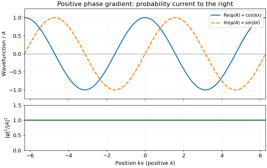
For the Schrödinger equation with a real scalar potential and no vector potential, the probability current isTogether with the probability density , it satisfies the continuity equation . Substituting givesA complex wavefunction requires both its real and imaginary parts in the sketch. Choosing the irrelevant constant phase so that is real, they are and , while the probability density is horizontal. It is the spatial phase gradient of a Schrodinger wavefunction that determines the sign of the probability current. In particular, and have the same real part but opposite probability currents, so the slope of the real part cannot determine the direction.
A nonzero plane wave on the whole real line is not square integrable. The displayed density is understood with box normalization, generalized normalization, or as a local description of a broad wave packet; it does not define a normalized probability distribution on the whole line.

In the scalar two-particle model, the fermionic exchange symmetry and bosonic exchange symmetry conditions areFor particles with spin, exchange acts on all their labels; the stated coordinate-only model fixes the spatial symmetry sector. Define . Equal masses make the kinetic operator invariant under exchange, and the assumed potential is invariant too, so . Therefore implies . The componentsare respectively symmetric and antisymmetric eigenfunctions whenever nonzero. Their sum is the original nonzero quantum state, so at least one is nonzero. An eigenspace may contain both sectors if the energy is degenerate.
The normal modes of two harmonically coupled identical particles provide the separation. The coordinate transformation to is orthogonal, with absolute Jacobian one. Exchanging the particles leaves fixed and changes to . Hence bosonic quantum states are even and fermionic quantum states odd in the relative coordinate. The chain rule givesAlso and . Combining the two trapping potentials with the interaction therefore gives the separated Hamiltonian operatorThese are independent oscillators of frequencies and . Both frequencies are positive in the stated range. Their product eigenstates have energiesThe parity of an oscillator level is . Consequently bosons allow even and fermions odd , while is unrestricted.
The bosonic ground state uses , and the fermionic ground state uses . The oscillator length in the relative mode isUsing the normalized Gaussian for each mode givesIndeed by differentiating the Gaussian, so it is the normalized odd first excited state. The ground energies are and .
Choose normalized factors for a normalized product quantum state; this can always be done by reciprocal rescaling of its factors. Since the coordinate Jacobian has absolute value one,If the supplied factors are not individually normalized, the general expression has an additional factor ; choosing normalized factors is the convention in the displayed formula.
For the ground states, put . Then and . Thus, for differentiable with suitable Gaussian integrability and vanishing boundary terms,This is integration by parts, and every polynomial satisfies the required endpoint conditions. The relative-coordinate moments in even and odd oscillator ground states follow by substituting :For odd , both expectations vanish by parity, so this is an equality of zeros rather than an increase in signed mean separation. The even moments show the physical difference. In particular and , so the fermionic root-mean-square particle separation is times the bosonic value. The fermionic probability density vanishes at coincidence , expressing Pauli exclusion principle in this spatial symmetry sector. This is an exchange constraint on the wave function, not an additional classical force. As approaches , the relative oscillator softens and its width diverges; the excluded endpoint would no longer have this normalizable oscillator ground state.
The Time-dependent Schrödinger equation, with the Hamiltonian for a particle of mass in a real potential energy , isA stationary state is an energy eigenstate: its wavefunction evolves by a single global phase,Its probability density is independent of time. For a normalized wavefunction, the probability density and probability current areSubtracting the complex conjugate of the Time-dependent Schrödinger equation, multiplied by , from the original equation multiplied by cancels the real potential energy terms and gives the continuity equation . Thus measures signed probability flow in the positive direction.
The initial quantum state is the equal superposition of the first two box states, . The orthonormality of the two energy eigenstates makes its squared norm equal to one. Their separate stationary state phases giveWrite . The probability density isEach squared sine integrates to on the left half. For the quantum interference term, the product-to-sum identity givesHence the Born rule givesThe quantum interference moves probability between the halves even though each component separately is a stationary state.
For a normalized wavefunction, the expectation value of a function of position isprovided the integral exists. For an unnormalized state, divide this expression by . Put . The ground state has probability density , which is even. ThusThe zero mean position expresses symmetry, whereas this positive expectation value measures the mean distance from the centre.
The time-independent Schrödinger equation is the energy eigenvalue equation for the Hamiltonian operator:Here is the reduced Planck constant. A corresponding stationary wavefunction evolves as , which follows by substitution in the Time-dependent Schrödinger equation. Its position probability density is time independent because the time factor has unit modulus. Physical energy eigenstates must also satisfy the system's boundary conditions; for a bound state, wavefunction normalization requires .
Write , and . Its derivative isIntegration by parts with the Dirichlet boundary conditions gives the energy expectationIt is constant in time, since the time-independent Hamiltonian operator has fixed energy measurement probabilities: .
For the midpoint parity operator, . Hence, again putting ,Indeed the imaginary part integrates to zero by reflection and . This expectation value is also constant in time, because the bounded self-adjoint operator commutes with and hence with its time-evolution operator. Equivalently, .
For the momentum operator, direct evaluation givesThe real sine-cosine integral vanishes. This expectation value is not constant in time: the infinite square well walls reverse motion. One can prove the change exactly without approximating the wavefunction. Atthe energy eigenstate expansion and give . Differentiation shows , soThis half revival in an infinite square well is a concrete counterexample to momentum conservation. The sign from is only a global phase.
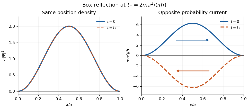

The apparent interior identity cannot justify conservation here: the momentum operator does not preserve the Dirichlet boundary conditions of the Hamiltonian operator's operator domain. For sufficiently regular states, retaining the boundary terms in Ehrenfest theorem instead gives the boundary force in an infinite square well,In the strictly confined interval, with both endpoint values zero is symmetric but not itself a self-adjoint operator. The requested integral is the conventional mean momentum; it also equals the full-line momentum mean of the zero-extended state, as measured upon releasing the walls. This domain distinction explains why the formal interior commutator misses the wall force.
The spatial quantum phase has unit modulus. Thus the probability density and total probability areThe exterior contributes zero. This establishes wavefunction normalization, although the spatial quantum phase means the state is not the ground energy eigenstate.
On a smooth wavefunction , the position operator and momentum operator giveThus the canonical commutation relation is . Since and are self-adjoint operators and are real, the adjoint operator of isExpanding the products in the stated order is essential:Subtracting gives . These identities initially hold on smooth rapidly decaying functions, which contain the quantum harmonic oscillator energy eigenstates used below.
The factorization also proves a lower bound: for a normalized energy eigenstate ,Therefore . The commutator product rule, applied to , givesSo a nonzero application of the creation operator raises the energy eigenvalue by , while the annihilation operator lowers it by the same amount.
Begin with any energy eigenstate, whose existence is assumed. Repeated lowering must terminate: otherwise it would eventually produce a nonzero energy eigenstate below , contradicting the lower bound. More explicitly, if with integer and , the first lowering steps are nonzero. If , one further step is also nonzero by its positive squared norm and has energy , an impossibility. Thus and the last state satisfies . This provesEvery level exists as well: , so repeated raising from never vanishes. The same factorization bounds the energy expectation of any normalized state in the one-dimensional harmonic oscillator form domain below by , proving that the terminated state really is a ground state.
To find its probability density, solve the first-order equationIts solutions are . With , the supplied Gaussian integral givesTaking fixes an irrelevant global phase. ConsequentlyThe ground-state energy is positive even though the potential minimum is zero: it is the oscillator's zero-point energy.
The identity gives the momentum eigenstate expansionUsing the orthonormal basis from part (a), the wavefunction normalization isHence . The wavefunction normalization leaves a global phase free; the positive real choice used in the requested expansion givesThe two nonzero eigenvalues of the momentum operator have the same energy eigenvalue . Under unitary time evolution, their coefficients acquire the same dynamical phase. With ,At , recovers the initial wavefunction. Its probability density, useful below, is
For a position measurement, the Born rule integrates the probability density over the chosen interval. The three terms from part (b) have integralsandThusThe oscillating term comes from quantum interference between the zero and positive energy components. The probability lies between and , both within ; integrating the same probability density over the whole circle gives one.
Put and retain the global phase from the preceding Lüders rule update. Since , the same orthonormal basis diagonalizes the new Hamiltonian operator, withIn particular, . Applying unitary time evolution from therefore givesThis is rigid translation from a momentum term in the Hamiltonian: the position probability density moves with velocity . The plus sign in follows directly from the negative sign of . At the expression agrees exactly with the preceding post-measurement state.
Apply the position version of the Born rule to the normalized wavefunction:The result is independent of because the state and the measurement interval scale together. Most position probability lies towards the right wall, since the probability density grows as .
The two probabilities concern different quantum measurements, so there is no requirement that they match or that one bound the other. The spatial interval contains little of the state: its probability density is smallest near zero and increases towards . By contrast, the positive ground state extends across the whole well. It has substantial same-sign overlap with the positive linear wavefunction, with no cancellation between lobes in the overlap integral. The right panel of the figure in solution illustrates these two amplitudes and marks the small position interval.
Consequently a large global ground-state probability can coexist with a small probability of finding the particle in the left third. This is not because the ground state is spatially confined to that third; a ground-state particle can be found throughout the well. In operator language the two events are projections onto a spatial subspace and onto one energy eigenstate, respectively.