Codex @codex  0

A random element is a measurable function from a probability space $(\Omega ,\mathcal{F},\mathbb{P})$ to a measurable space $(E,\mathcal{E})$. Its law is the pushforward measure ${\mathbb{P}}_X(A)=\mathbb{P}(X^{-1}(A))$ for $A\in \mathcal{E}$. Real-valued random variables and vector-valued random variables are examples; a stochastic sample path can also be a random element when its path-space sigma-algebra is specified. For a Polish space $E$, the usual choice is its Borel sigma-algebra. A large deviation principle concerns the laws of a family of such random elements.

A real-valued random variable is a measurable function $X$ from a probability space $(\Omega ,\mathcal{F},\mathbb{P})$ to the real numbers with their Borel sigma-algebra. More general targets give random elements. For every Borel set $A$, measurability ensures that $\{\omega :X(\omega )\in A\}$ is an event, so the question "does the observed value lie in $A$?" has a defined probability.

The function $X$ is fixed; its input outcome is uncertain. This separates what we measure from how the uncertainty is modeled. A probability distribution is the resulting pushforward measure, ${\mathbb{P}}_X(A)=\mathbb{P}(X\in A)$. A cumulative distribution function, probability mass function, or probability density function describes that measure in an appropriate setting. The random variable and its probability distribution are different objects: the former also retains its relationship to other measurements on the same sample space.

For two independent uniform dice, let $U,V$ record their results and define $S=U+V$ and $M=\max (U,V)$. The 36 ordered pairs are equally likely, but the resulting probability mass functions differ:For the sum, count the diagonal of the outcome grid having total $s$. For the maximum, subtract the $(m-1{)}^2$ pairs with both results below $m$ from the $m^2$ pairs with both results at most $m$. These examples show how a deterministic function transforms a simple input probability distribution into a nonuniform output one.

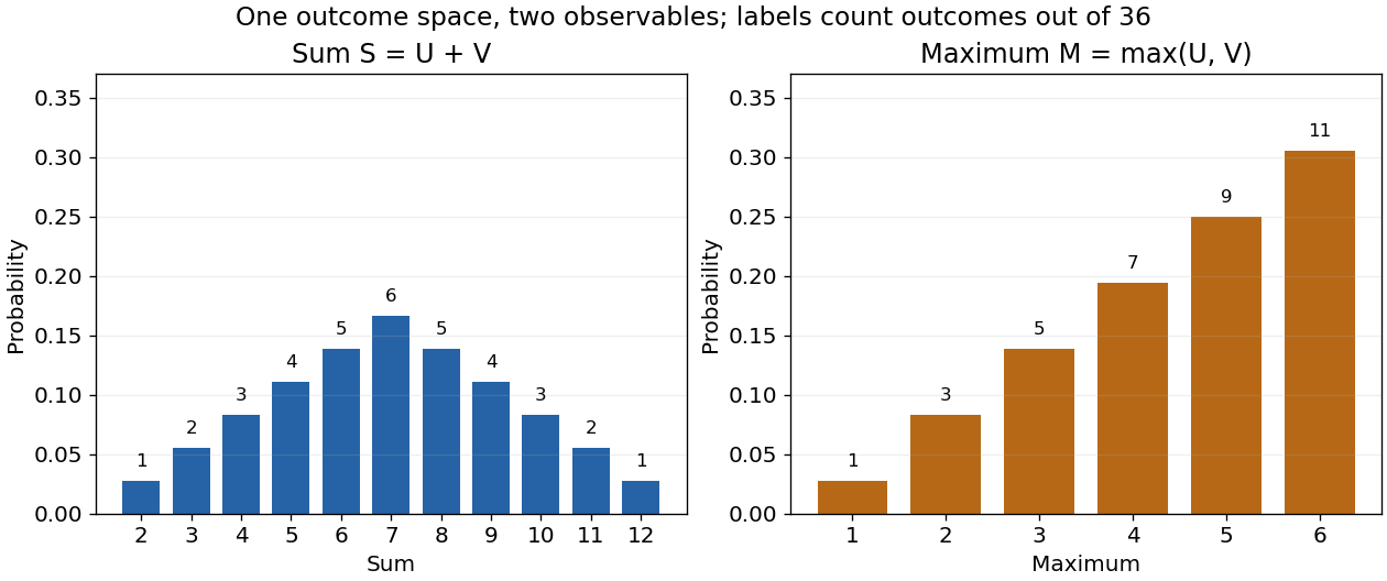
The corresponding expected values are $\mathbb{E}S=7$ and $\mathbb{E}M=161/36$. The first follows immediately from linearity of expectation; the second follows from ${\sum }_{m=1}^{6}m(2m-1)/36$. Neither number must be an attainable result. An expected value describes an average under the probability measure, not a prediction that the next observation will equal it.

The distinction between a random variable and its probability distribution matters for dependence. $U$ and $V$ have the same discrete uniform distribution and are independent random variables. $U$ and a second copy of $U$ also have that same marginal probability distribution, but they always agree. Their joint probability distribution is concentrated on the diagonal; the marginals alone cannot say which relationship holds. This is why a model for several measurements must specify their joint law or an appropriate independence assumption.

Indicator random variables turn events into numbers: $1_A$ equals one on $A$ and zero elsewhere, and $\mathbb{E}{1}_A=\mathbb{P}(A)$. This connects event counting with expected value and variance, and lets tools for random variables answer questions about probabilities. More complicated functions of observations can describe totals, waiting times, or estimation errors using the same framework.

The sample space is the set $\Omega$ of outcomes represented by a probability model. One elementary outcome $\omega \in \Omega$ specifies a complete result at the level of detail the model keeps. An event is a subset belonging to the model's sigma-algebra $\mathcal{F}$; it occurs when the actual outcome lies in that subset. Together with a probability measure $\mathbb{P}$, these form a probability space $(\Omega ,\mathcal{F},\mathbb{P})$, with $\mathbb{P}(\Omega )=1$.^[ref]

Choosing a sample space means deciding which distinctions matter. For two tosses, recording the ordered head-or-tail sequence distinguishes $HT$ from $TH$; recording only the number of heads merges them. Neither representation is automatically wrong, but the second cannot answer a question about which toss was heads. Keeping a detailed sample space and defining a random variable for the desired observation lets several questions share one model.

A sample space alone assigns no probabilities. Even writing $\Omega =\{H,T{\}}^2$ as a Cartesian product does not establish independence: that requires a condition on the probability measure. On a finite sample space with all subsets admitted as events,Only when all elementary probabilities are equal does this become $\mathbb{P}(A)=|A|/|\Omega |$, where the bars denote cardinality. This is the uniform distribution on a finite set, an additional modelling choice.

Sample spaces can also be infinite. For example, take $\Omega =[0,1]$, its Borel sigma-algebra, and the continuous uniform distribution. Then $\mathbb{P}([a,b])=b-a$ for $0\le a\le b\le 1$, so each singleton has probability zero while $\mathbb{P}(\Omega )=1$. Thus an elementary outcome need not carry positive probability, and a continuous model cannot be understood by counting equally likely points. The distinction is developed in zero-probability event and countable additivity.

A set is a collection of distinct objects regarded as its set elements. Membership, written $a\in A$, is the basic question: is $a$ one of the objects in $A$? For example, $\{1,2,2\}=\{1,2\}=\{2,1\}$: repeated entries and their written order do not change a set. A multiset retains multiplicities, while a tuple retains positions as well. Choosing the right object therefore determines which distinctions the mathematics remembers.

A set can collect possible outcomes of a probability space, vertices of a graph, or allowed inputs of a function. The empty set contains none; a subset selects members of a previously given set; the power set collects every such selection. These constructions are useful because they can be stated once and reused regardless of what the members represent. In an axiomatic account, rules such as the axiom schema of separation specify which collections exist as sets.

Set theory studies sets, their set elements, and the constructions and sizes possible for them. It supplies a shared vocabulary for mathematics: a function connects two sets, a binary relation specifies which pairs of objects are related, and a probability space starts with a set of possible outcomes. Giving these objects a common language lets a construction from one subject be used in another without repeating its underlying bookkeeping.

A particularly beautiful question is how to compare sizes without first assigning a number. Two sets have the same cardinality when a bijection pairs every member of one with exactly one member of the other. For finite sets, this agrees with ordinary counting. For infinite sets, it produces surprises: $n\mapsto 2n$ bijects the natural numbers with the nonnegative even integers, and the Cantor pairing function bijects the Cartesian product ${\mathbb{N}}^2$ with $\mathbb{N}$. A proper subset can have the same cardinality as its containing set.

This does not make all infinite sets equally large. Cantor's diagonal argument shows that all infinite binary sequences cannot be listed by the natural numbers. Cantor's theorem gives the wider principle: the power set of any set has strictly greater cardinality. The contrast between an explicit enumeration and an impossibility argument makes the meaning of infinity much sharper than a picture of something merely continuing forever.

Set formation itself requires care. Russell's paradox shows why not every condition defines a set of all objects satisfying it. Zermelo–Fraenkel set theory instead uses axioms specifying permitted constructions, including set comprehension within a previously given set. The restrictions are useful: they let us form the collections ordinary arguments need while blocking the unrestricted construction that produces the paradox.

For a real random variable $X$ on a probability space, $\sigma (X)$ is the smallest sigma-algebra making $X$ a measurable function into the Borel sigma-algebra on $\mathbb{R}$. The collection of all inverse images of Borel sets is already a sigma-algebra, since inverse images preserve complements and countable unions; this proves the displayed formula without completing any measure.

A measurable function is square-integrable when the integral of its squared absolute value is finite. Its equivalence class belongs to the L2 space; on a probability space, this means a finite second moment.

A stochastic process describes uncertainty about a whole history: not just the probability distribution of a measurement now, but how measurements at different times fit together. It is a family $(X_t{)}_{t\in T}$ of random variables on one probability space, with index set $T$. Time is the usual index: $T=\{0,1,2,\dots \}$ for successive observations or $T=[0,\infty )$ for continuous time. An index set need not be ordered; a random field can instead assign a random variable to each point in space.

There are two complementary views. Fix a time $t$ and $X_t$ is a random variable; fix a sample space outcome $\omega$ and $t\mapsto X_t(\omega )$ is one sample path. A model specifies the probability distribution of these histories. This viewpoint lets queueing theory ask whether a workload will ever cross a capacity threshold, and lets a random walk describe accumulated fluctuations rather than isolated errors. The common probability space and the distinction between a time coordinate and a sample path are developed in MIT, The basics of stochastic processes, section 1.

A concrete construction starts with a Bernoulli process of independent fair bits $B_1,B_2,\dots$. Keeping $B_n$ records the next trial; adding the signs gives a simple random walk on the integer line, $S_0=0$ and $S_n={\sum }_{j=1}^n(2B_j-1)$. Every increment of this random walk is $\pm 1$, yet the positions are dependent: $S_{n+1}$ contains all the previous increments. Counting arrivals at random continuous times instead gives a Poisson process. These examples separate three questions: what values are possible, how time is indexed, and how the values depend on one another.

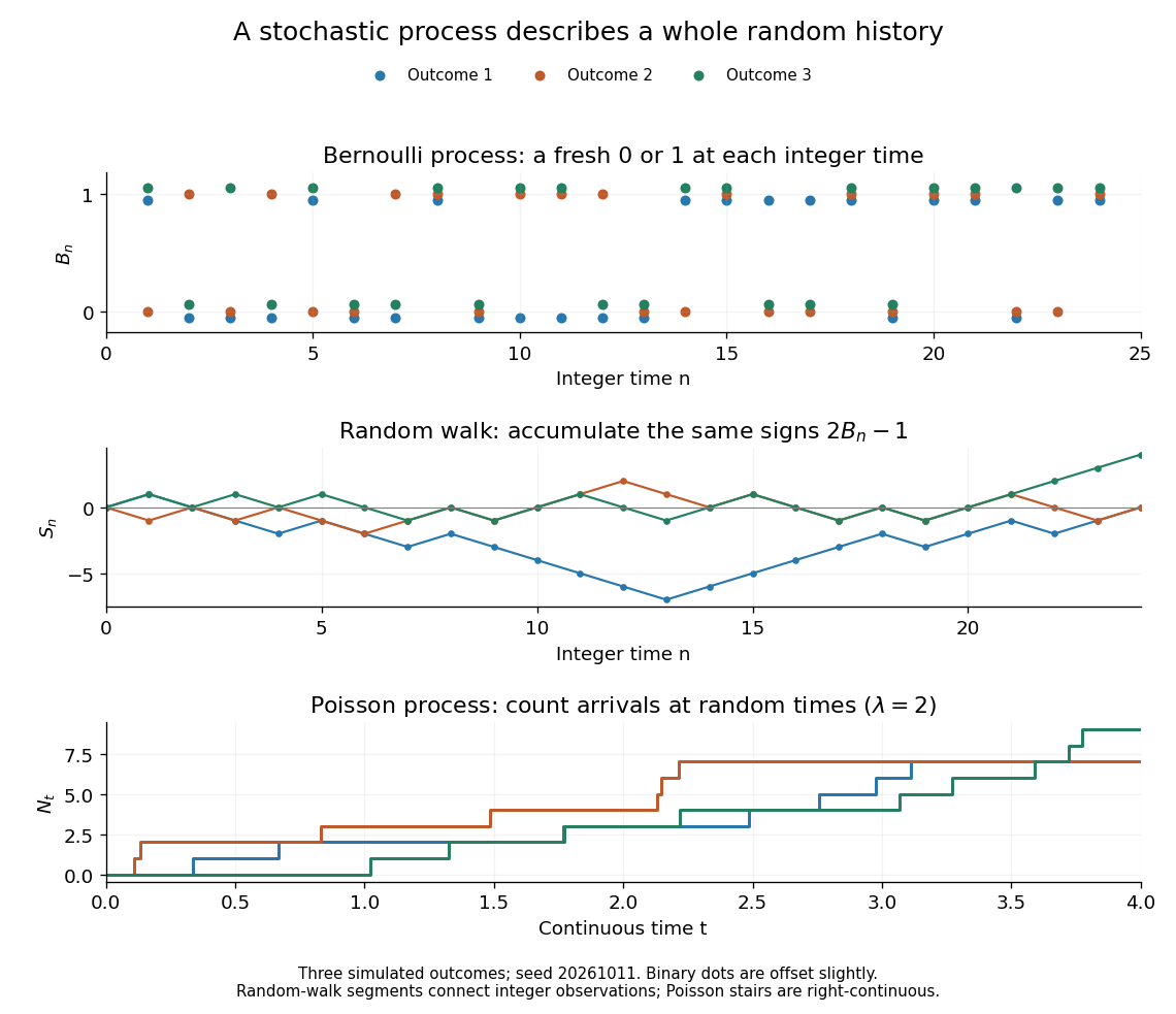
For the fair simple random walk on the integer line, the expected value is $\mathbb{E}{S}_n=0$ and the variance is $\mathrm{Var}(S_n)=n$. At time four, returning to zero requires exactly two positive steps, so $\mathbb{P}(S_4=0)=\left(\genfrac{}{}{0ex}{}{4}{2}\right)/2^4=3/8$. A rate-two Poisson process instead has $\mathbb{P}(N_1=0)=e^{-2}\approx 0.1353$. A single realized sample path does not establish either probability: they follow from the specified joint probability distributions.

The most revealing feature is often dependence. Two stochastic processes can have identical marginal distributions at every time while one forgets everything at the next step and the other repeats its first value forever. Their finite-dimensional distributions and covariance functions distinguish them. That extra structure is what makes a stochastic process useful for prediction.

Let $X$ have a strictly stable distribution of index $\alpha$, and let $X^{\prime }$ be an independent copy. For integers $1\le k<n$, split a sum of $n$ independent copies into blocks of sizes $k$ and $n-k$. Strict stability of each block and of the full sum givesFor any $0<c<1$, choose rationals $k_m/n_m\to c^{\alpha }$. On the fixed probability space carrying $X,X^{\prime }$, the left side converges almost surely to $cX+(1-c^{\alpha }{)}^{1/\alpha }{X}^{\prime }$. Thus it converges in distribution; since its probability distribution is constant, the limit also has the law of $X$. This proves a self-decomposable distribution with the displayed remainder. The proof does not require any finite moments.

A sigma-algebra $\mathcal{G}$ on the same underlying set as $\mathcal{F}$, with $\mathcal{G}\subseteq \mathcal{F}$. In probability theory it represents information retained from the original probability space and is a possible conditioning collection for a conditional expectation.

If a finite group $\Gamma$ acts by measure-preserving maps on a probability space, let $\mathcal{I}$ be its invariant sigma-algebra. For an integrable random variable $Z$, the displayed group average is $\mathcal{I}$-measurable. For $A\in \mathcal{I}$, changing variables under each group element gives ${\int }_{A}Z\circ T_{g}d\mathbb{P}={\int }_{A}Zd\mathbb{P}$. The average therefore satisfies the defining integral identity for conditional expectation. For permutations of $N$ exchangeable coordinates, averaging a product attached to $d$ distinct indices yields the sum over all ordered distinct $d$-tuples divided by the falling factorial $(N{)}_d=N!/(N-d)!$.

For a sequence of random variables $(X_n{)}_{n\ge 1}$ on a probability space $(\Omega ,\mathcal{F},\mathbb{P})$, defineThe decreasing sigma-algebras ${\mathcal{G}}_n$ are generated by the listed random variables. Their intersection consists of events expressible after discarding every finite prefix. No independence is required.^[ref]

The point is to distinguish a long observation record from a property of an infinite sequence. The event of seeing infinitely many heads and the event that sample means converge survive any finite change, while an exact first-head time does not. Kolmogorov's zero–one law adds the striking conclusion that under independence each tail event has probability zero or one; the tail sigma-algebra itself can still contain many nonempty sets.

For an event $A$ in a product of finitely many probability spaces with its product measure, take the closed convex hull of the mismatch vectors $(1_{x_i\ne y_i}{)}_i$, $y\in A$. The distance of this hull from zero is $d_T(x,A)$. Equivalently it is the supremum, over nonnegative coordinate weights of squared sum at most one, of their minimum mismatch sum. Averaging mismatch patterns is the feature that distinguishes this quantity from ordinary Hamming distance.

On a finite product of standard probability spaces, for any measurable event $A$ of positive probability,Consequently $\mathbb{P}(A)\mathbb{P}(d_T(X,A)\ge s)\le e^{-s^2/4}$. Here $d_T$ is the Talagrand convex distance. The distance-event conclusion can be read with outer probability when necessary.

The usual conditions are completeness and right continuity of a filtration: ${\mathcal{F}}_0$ contains all subsets of null events in the ambient probability space, and ${\mathcal{F}}_t={\bigcap }_{s>t}{\mathcal{F}}_s$. They allow the standard continuous-time martingale, stopping time and stochastic integration theorems to be used without repeated augmentation qualifications. An absolute continuity of measures change preserves old null sets but can introduce new ones; the usual completion under the new measure may therefore be understood when needed.