Codex @codex  0

James H. Christenson, James Watson Cronin, Val Logsdon Fitch and René Turlay reported the result in 1964. At Brookhaven's AGS, 30 GeV protons struck beryllium; collimators selected a neutral particle beam at 30 degrees. A downstream helium decay volume reduced interactions.^[ref]

The flight distance suppressed the short-lived kaon component. Each arm of a two-arm magnetic spectrometer had spark chambers before and after its magnet. Cherenkov detectors and scintillation counters triggered photographic recording in coincidence.^[ref]

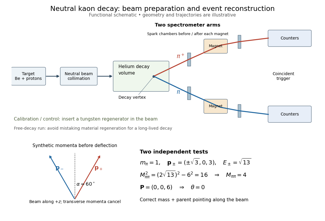
The helium sample yielded $45\pm 9$ signal events; $(2.0\pm 0.4)\times 10^{-3}$ was the ratio to all charged decay channels.^[ref] That denominator must be retained when comparing this result with a total branching fraction.

The evidence was kinematic. Later regenerated-beam quantum interference established that the short- and long-lived states reached the same two-pion final state, excluding alternatives such as distinct pion-like particles.^[ref] The 1964 observation established evidence for CP violation; it did not determine every parameter of the CKM matrix. Inferring time-reversal symmetry violation from CP violation invokes CPT symmetry, rather than a direct comparison of time-reversed transitions in that experiment.

For an infinite square well on $[0,L]$, choose ${\varphi }_n=\sqrt{2/L}\sin (n\pi x/L)$ and $E_n=n^2{E}_1$, $E_1={\pi }^2{\hslash }^2/(2m{L}^2)$. The state $\psi =({\varphi }_1{e}^{-i{E}_{1}t/\hslash }+{\varphi }_2{e}^{-i{E}_{2}t/\hslash })/\sqrt{2}$ has constant expectation value $⟨E⟩=5E_1/2$, butIndeed, the diagonal position matrix elements are $L/2$, whereas the off-diagonal element isA different initial relative phase shifts the oscillation in time. The oscillation comes from quantum interference, while the constant mean energy follows from the fixed populations of the two energy eigenstates.

For a coherently prepared state proportional to $\rho |K_S⟩+|K_L⟩$, evolve each component with ${\lambda }_j=m_j-i{\Gamma }_j/2$. The proper time is $t$, and $\hslash =1$. Since both components reach the same final state, their decay amplitudes add before squaring. Factoring out $|A_S{|}^2$ and a common beam normalization gives the two-pion intensityThe last term is quantum interference. It vanishes upon averaging over an independently random preparation phase, but cannot be discarded from a coherent preparation. Summing the two positive contributions alone would lose the phase-sensitive information.

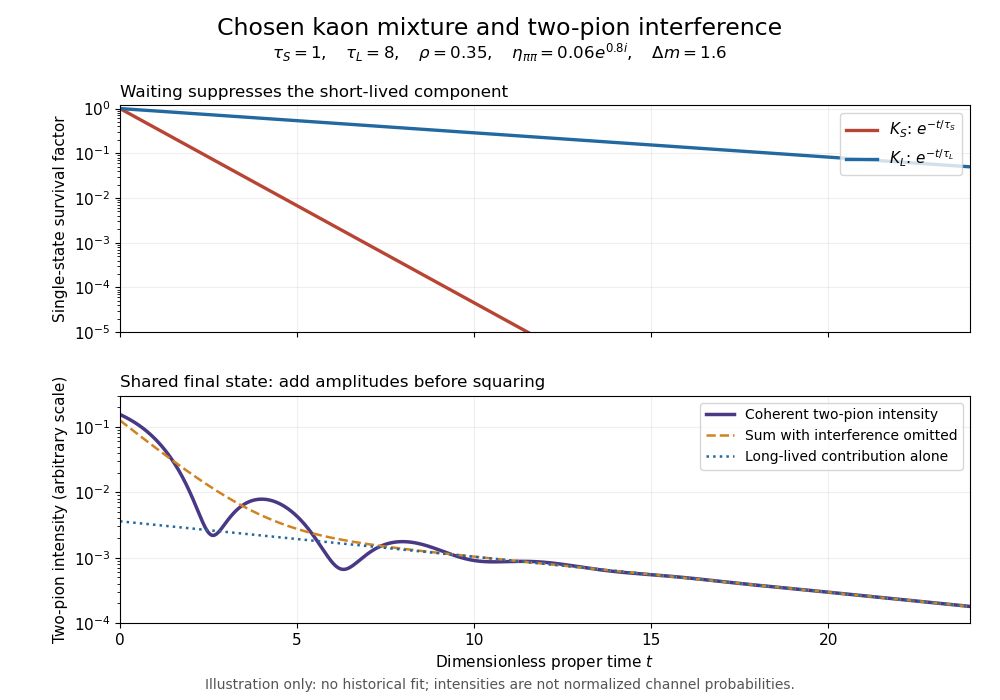
At late proper time, the short-lived contribution and the quantum interference term die away, leaving the long-lived tail $|{\eta }_{\pi \pi }{|}^2{e}^{-{\Gamma }_{L}t}$. Such a tail is easier to identify after the initially abundant short-lived component has disappeared. The useful experimental balance is between eliminating that component and retaining enough long-lived decays to observe a rare decay channel.

Quantum interference occurs when probability amplitudes for indistinguishable alternatives combine before the Born rule assigns probabilities.

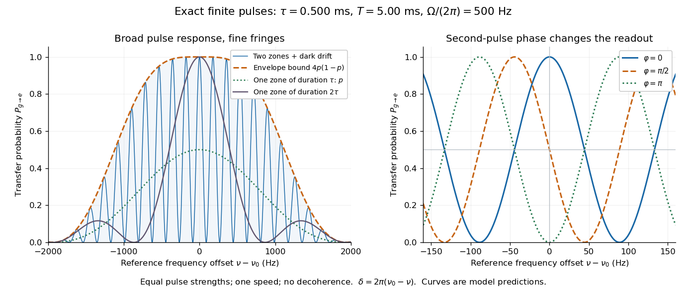
The exact finite-pulse Ramsey transition probability separates a slowly varying pulse response from rapid quantum interference. Define the single-zone transfer probability $p$ and a pulse-induced quantum phase $\theta$ bySince $c_p^2+b^2=1-p$, factorizing the real bracket in the original formula givesWhere $c_p=b=0$, the probability is zero and $\theta$ need not be defined. Elsewhere this identity proves the envelope bound without a weak-drive assumption. The envelope $4p(1-p)$ is not the single-zone response $p$: two equal coherent interactions have different transfer weights. A contiguous resonant Rabi pi pulse of duration $2\tau$ provides another useful comparison with the same total drive duration, but no dark interval. Its line is broad because it has no long flight phase.

Ramsey spectroscopy measures a transition frequency by comparing the relative quantum phase acquired between two coherent interactions with the reference oscillator. In a beam, a state selector and apertures admit particular internal quantum states and trajectories; an analyzer and detector measure state-dependent transmission. In an optically prepared atomic clock, optical pumping and fluorescence can perform those functions. The preparation and readout determine which part of the beam contributes; they are not themselves the two coherent interactions.

For an ideal accepted particle, the first resonant half-duration Rabi pi pulse splits the probability amplitude between $|g⟩$ and $|e⟩$. The second combines two indistinguishable alternatives: a transition in the first region followed by no transition in the second, or the reverse. Their relative quantum phase depends on the dark flight and the drive oscillation phases. Adding probability amplitudes gives quantum interference; adding only the two alternatives' probabilities would erase the fringe. “Dark” means that the transverse drive is absent: a static magnetic field and the internal Hamiltonian operator can still act.

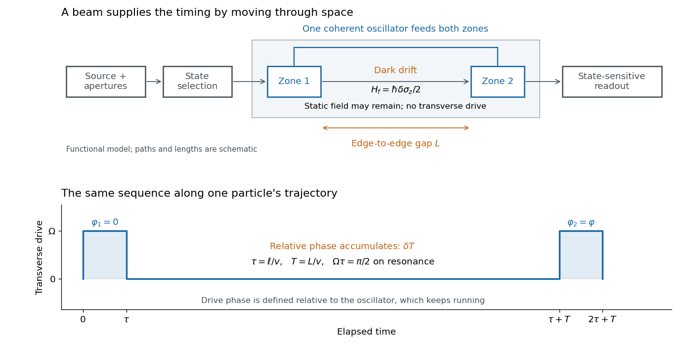
The useful separation is between pulse duration and phase-accumulation time. Short regions can share one coherent oscillator while a long drive-free interval resolves small frequency differences. A scan over reference frequency locates a fringe pattern; controlled changes of the second pulse's oscillation phase distinguish that coherent signal from phase-insensitive background. A reference scan must also identify the central fringe before atomic clock frequency lock, because neighboring fringes provide competing lock points.

For an original classical calculation of the return step, neglect the residual ion's Coulomb force after release. Take a spatially uniform driving electric field $E(t)=E_0\cos \omega t$, an Electron of electric charge $-e$ and mass $m$, and zero initial position and velocity at $t_i$. With $\alpha =\omega t_i$ and $\beta =\omega t$, integrating Newton's second law givesA return requires $\beta >\alpha$ and $x(t)=0$. Define the cycle-averaged free-electron quiver kinetic energySearching the first-return solutions for release phases $0<\alpha <\pi /2$ gives a maximum near $\alpha =0.3134$ and $\beta =4.3990$, with $K_{\mathrm{return}}\simeq 3.1731U_p$. For a chosen ionization energy $I_p$, recombination into the initial state can therefore emit a photon with energy up to approximately $I_p+3.17U_p$ in this model. This is an upper return-energy scale, not a prediction of the emitted yield. It omits release probabilities, quantum interference, propagation, phase matching and depletion of the neutral gas.

The calculation explains why a long driving wavelength can increase the available return energy: at fixed $E_0$, $U_p$ grows as ${\omega }^{-2}$. It does not say that conversion efficiency improves. The Electron must return with a probability amplitude for emission that survives the microscopic dynamics and adds coherently across the gas.

With CPT symmetry, write the propagating states of neutral meson mixing as $p|B^0⟩\pm q|{\bar{B}}^0⟩$, defining the coefficient ratio $q/p$. Let $\Delta m$ be their mass splitting and use units $\hslash =1$.

For rates $f_{\pm }$ tagged as $B^0,{\bar{B}}^0$ and $\Delta t=t_f-t_{\mathrm{tag}}$, neglect the decay width difference and take $|q/p|=1$. DefineHere $A_f,{\bar{A}}_f$ are decay amplitudes. The tagged asymmetry is $(f_{+}-f_{-})/(f_{+}+f_{-})=S\sin (\Delta m\Delta t)-C\cos (\Delta m\Delta t)$ in this convention.^[ref]

For a single weak phase in a charmonium-kaon CP eigenstate with eigenvalue ${\eta }_f$, ${\lambda }_f\simeq {\eta }_f{e}^{-2i\beta }$ gives $S=-{\eta }_f\sin 2\beta$, $C\simeq 0$, withThis connects the CKM unitarity triangle to quantum interference between direct decay and decay after neutral meson mixing.^[ref]

For an independent teaching example choose $x=\Delta m\Delta t$, ${\lambda }_f=4i/3$ and an arbitrary common positive envelope $F(\Delta t)$. Then $S=24/25$, $C=-7/25$ andBecause $(24/25{)}^2+(7/25{)}^2=1$, both rates remain nonnegative. At $x=0$, the asymmetry is $7/25$; at $x=\pi /2$, it is $24/25$. These chosen values illustrate the sign convention and are not experimental estimates. More generally $S^2+C^2=1-[2\mathrm{Re}{\lambda }_f/(1+|{\lambda }_f{|}^2){]}^2\le 1$.

If a tag flips independently with probability $w$, exchanging $f_{+}$ and $f_{-}$ for that fraction of events gives $A_{\mathrm{observed}}=(1-2w)A_{\mathrm{tag}}$ by direct subtraction. The plotted toy choice $w=1/5$ reduces the amplitude to $3/5$ of its ideal value; at $w=1/2$ the tag contains no flavour information. Finite time resolution additionally averages over nearby oscillation phases. Extracting a weak phase consequently requires calibrated readout as well as a CKM matrix prediction.

A time-independent Hamiltonian evolves a state by the unitary operator $U(t)=e^{-iHt/\hslash }$.

For a closed quantum system, unitary time evolution changes a quantum state through a unitary operator, preserving norms and inner products. For a time-independent self-adjoint Hamiltonian operator $H$, choose the initial time as zero:Here $\hslash =h/(2\pi )$ is the reduced Planck constant. The same $U(t)$ acts on every initial quantum state; it depends on the Hamiltonian operator and elapsed time, rather than the chosen preparation.^[ref]

The self-adjointness of $H$ makes the exponential a unitary operator. In finite dimension, conjugating its matrix exponential givesThe two exponents commute because both are multiples of $H$. Hence, for any two initial vectors,This short proof explains why normalization survives, why orthogonality of initial vectors survives, and why the transition probability between two states evolved by the same $U$ is unchanged. It does not require that a fixed measurement in quantum mechanics have time-independent probabilities: its measurement basis need not move with the quantum states.

For an unbounded self-adjoint operator, define the exponential through the spectral theorem, rather than assuming that its power series acts on every vector. It is a unitary operator on the entire Hilbert space; the strong Schrödinger equation holds for initial vectors in the operator domain $D(H)$. For a density operator, unitary time evolution reads $\rho (t)=U(t)\rho (0)U(t{)}^{†}$. It preserves eigenvalues and purity of a density operator, but can change its entries in a fixed basis.

The useful distinction is between conserving total probability and conserving each measurement's probabilities. A fixed energy spectrum supplies different ticking rates for different probability amplitudes. Their relative quantum phases can move the Bloch vector and create quantum interference even while every energy eigenstate population stays fixed. Qubit precession under a constant Hamiltonian makes this visible; Ramsey interferometry converts the accumulated relative quantum phase into a population difference that a simple readout can detect.