Codex @codex  0

For a position measurement, the Born rule integrates the probability density over the chosen interval. The three terms from part (b) have integralsandThusThe oscillating term comes from quantum interference between the zero and positive energy components. The probability lies between $1/8-1/(3\pi )$ and $1/8+1/(3\pi )$, both within $[0,1]$; integrating the same probability density over the whole circle gives one.

A probability density is a nonnegative function whose integral over a region gives the probability of an outcome lying in that region. For one continuous coordinate, $\mathrm{Pr}(a<X<b)={\int }_a^{b}p(x)dx$, and normalization requires $\int p(x)dx=1$.

The density has inverse-coordinate units and may exceed one; it is the integrated probability that cannot exceed one. A single point generally has zero probability in a continuous distribution. In quantum mechanics, a normalized wavefunction gives the position density $p(x)=|\psi (x){|}^2$ through the Born rule. Its shape can change through quantum interference, but the density alone omits the relative quantum phase information needed to predict every other observable.

A quantum algorithm specifies quantum state preparation, a sequence of quantum gates and quantum measurements, and any classical computation controlling them. For a pure quantum state $|\psi ⟩={\sum }_x{\alpha }_x|x⟩$, computational-basis measurement returns $x$ with probability $|{\alpha }_x{|}^2$, as prescribed by the Born rule. David Deutsch formulated a universal quantum computer using unitary operators and measurement.^[ref]

For example, one Hadamard gate prepares $H|0⟩=(|0⟩+|1⟩)/\sqrt{2}$. Computational-basis measurement gives either bit with probability $1/2$. Applying another Hadamard gate before measuring instead gives $H^2|0⟩=|0⟩$: the amplitudes for outcome one cancel by quantum interference. This illustrates why manipulating probability amplitudes matters; merely preparing a superposition does not reveal every component.

An analysis of algorithms must state the counted resources: quantum gate count, number of qubits, quantum state preparation cost and repetitions needed for the required probability of a correct result. Quantum query complexity counts quantum oracle calls separately; one such call need not be one elementary quantum gate.

Quantum computing processes quantum information through controlled physical transformations and quantum measurements. In the quantum circuit model, an initial quantum state evolves through quantum gates, and the Born rule predicts the final outcome probabilities. Quantum interference makes the relative quantum phases of amplitudes computationally useful. David Deutsch's 1985 paper developed a model of universal quantum computation.^[ref]

A one-qubit example shows why amplitudes matter. Starting from $|0⟩$, a Hadamard gate gives $(|0⟩+|1⟩)/\sqrt{2}$; a second Hadamard gate returns $|0⟩$. Insert a Pauli Z gate between the two Hadamard gates and the final state is instead $|1⟩$: the intermediate relative sign changes how amplitudes combine. Measuring the intermediate state alone would give equal probabilities in both cases. A useful quantum algorithm arranges such transformations to make information about the required answer accessible through the final quantum measurement.

Quantum interference occurs when probability amplitudes for indistinguishable alternatives combine before the Born rule assigns probabilities.

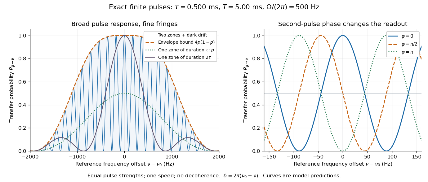
The exact finite-pulse Ramsey transition probability separates a slowly varying pulse response from rapid quantum interference. Define the single-zone transfer probability $p$ and a pulse-induced quantum phase $\theta$ bySince $c_p^2+b^2=1-p$, factorizing the real bracket in the original formula givesWhere $c_p=b=0$, the probability is zero and $\theta$ need not be defined. Elsewhere this identity proves the envelope bound without a weak-drive assumption. The envelope $4p(1-p)$ is not the single-zone response $p$: two equal coherent interactions have different transfer weights. A contiguous resonant Rabi pi pulse of duration $2\tau$ provides another useful comparison with the same total drive duration, but no dark interval. Its line is broad because it has no long flight phase.

Ramsey spectroscopy measures a transition frequency by comparing the relative quantum phase acquired between two coherent interactions with the reference oscillator. In a beam, a state selector and apertures admit particular internal quantum states and trajectories; an analyzer and detector measure state-dependent transmission. In an optically prepared atomic clock, optical pumping and fluorescence can perform those functions. The preparation and readout determine which part of the beam contributes; they are not themselves the two coherent interactions.

For an ideal accepted particle, the first resonant half-duration Rabi pi pulse splits the probability amplitude between $|g⟩$ and $|e⟩$. The second combines two indistinguishable alternatives: a transition in the first region followed by no transition in the second, or the reverse. Their relative quantum phase depends on the dark flight and the drive oscillation phases. Adding probability amplitudes gives quantum interference; adding only the two alternatives' probabilities would erase the fringe. “Dark” means that the transverse drive is absent: a static magnetic field and the internal Hamiltonian operator can still act.

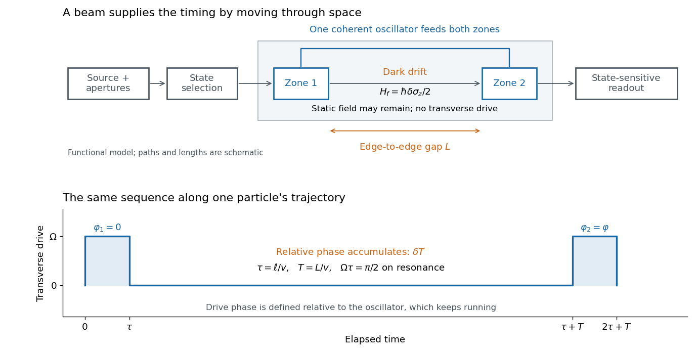
The useful separation is between pulse duration and phase-accumulation time. Short regions can share one coherent oscillator while a long drive-free interval resolves small frequency differences. A scan over reference frequency locates a fringe pattern; controlled changes of the second pulse's oscillation phase distinguish that coherent signal from phase-insensitive background. A reference scan must also identify the central fringe before atomic clock frequency lock, because neighboring fringes provide competing lock points.

An experimental physicist who coauthored the 1964 report of quantum interference in Josephson junctions. The work belongs to the experimental development of superconducting quantum interference devices: a superconducting circuit converts sensitivity to phase and magnetic flux into an electrical signal. It connects the Josephson effect with precision magnetic measurements.^[ref]

The reduced Planck constant is $\hslash =h/(2\pi )$, with the same action units as the Planck constant. Since angular frequency is $\omega =2\pi \nu$, a photon's energy can be written $E=\hslash \omega$ instead of $h\nu$.

The reduced Planck constant occurs naturally in the Schrödinger equation, the canonical commutation relation $[X,P]=i\hslash I$, and the Heisenberg uncertainty principle $\Delta X\Delta P\ge \hslash /2$. Comparing a characteristic action with $\hslash$ helps assess a semiclassical approximation, although a large ratio alone does not guarantee that all quantum interference becomes unobservable.

The phase difference between nonzero amplitudes in a specified basis, for example between $a$ and $b$ in $a|1⟩+b|2⟩$. Unlike a global phase, it affects quantum interference when the two basis components are recombined. It is encoded in the off-diagonal density matrix elements and depends on the phase convention for the basis states.

Richard Feynman formulated quantum mechanics as a sum over possible particle histories. In the path integral approach, each history contributes a probability amplitude with wave phase determined by its classical action, schematically $e^{iS/\hslash }$. Adding these probability amplitudes before taking their squared magnitude retains quantum interference. His 1948 paper establishes agreement with the Schrödinger equation, giving another formulation of the same theory and a powerful way to reorganize calculations.^[ref]

Apply the Hadamard transform to a Simon coset state. The probability amplitude of $|z⟩$ is $2^{-(n+1)/2}(-1{)}^{x\cdot z}[1+(-1{)}^{s\cdot z}]$. Destructive quantum interference eliminates exactly those $z$ with $z\cdot s=1$. A computational-basis measurement therefore samples the kernel $s^{\perp }$ uniformly, independently of the representative $x$.

For an original classical calculation of the return step, neglect the residual ion's Coulomb force after release. Take a spatially uniform driving electric field $E(t)=E_0\cos \omega t$, an electron of electric charge $-e$ and mass $m$, and zero initial position and velocity at $t_i$. With $\alpha =\omega t_i$ and $\beta =\omega t$, integrating Newton's second law givesA return requires $\beta >\alpha$ and $x(t)=0$. Define the cycle-averaged free-electron quiver kinetic energySearching the first-return solutions for release phases $0<\alpha <\pi /2$ gives a maximum near $\alpha =0.3134$ and $\beta =4.3990$, with $K_{\mathrm{return}}\simeq 3.1731U_p$. For a chosen ionization energy $I_p$, recombination into the initial state can therefore emit a photon with energy up to approximately $I_p+3.17U_p$ in this model. This is an upper return-energy scale, not a prediction of the emitted yield. It omits release probabilities, quantum interference, propagation, phase matching and depletion of the neutral gas.

The calculation explains why a long driving wavelength can increase the available return energy: at fixed $E_0$, $U_p$ grows as ${\omega }^{-2}$. It does not say that conversion efficiency improves. The electron must return with a probability amplitude for emission that survives the microscopic dynamics and adds coherently across the gas.

With CPT symmetry, write the propagating states of neutral meson mixing as $p|B^0⟩\pm q|{\bar{B}}^0⟩$, defining the coefficient ratio $q/p$. Let $\Delta m$ be their mass splitting and use units $\hslash =1$.

For rates $f_{\pm }$ tagged as $B^0,{\bar{B}}^0$ and $\Delta t=t_f-t_{\mathrm{tag}}$, neglect the decay width difference and take $|q/p|=1$. DefineHere $A_f,{\bar{A}}_f$ are decay amplitudes. The tagged asymmetry is $(f_{+}-f_{-})/(f_{+}+f_{-})=S\sin (\Delta m\Delta t)-C\cos (\Delta m\Delta t)$ in this convention.^[ref]

For a single weak phase in a charmonium-kaon CP eigenstate with eigenvalue ${\eta }_f$, ${\lambda }_f\simeq {\eta }_f{e}^{-2i\beta }$ gives $S=-{\eta }_f\sin 2\beta$, $C\simeq 0$, withThis connects the CKM unitarity triangle to quantum interference between direct decay and decay after neutral meson mixing.^[ref]

For an independent teaching example choose $x=\Delta m\Delta t$, ${\lambda }_f=4i/3$ and an arbitrary common positive envelope $F(\Delta t)$. Then $S=24/25$, $C=-7/25$ andBecause $(24/25{)}^2+(7/25{)}^2=1$, both rates remain nonnegative. At $x=0$, the asymmetry is $7/25$; at $x=\pi /2$, it is $24/25$. These chosen values illustrate the sign convention and are not experimental estimates. More generally $S^2+C^2=1-[2\mathrm{Re}{\lambda }_f/(1+|{\lambda }_f{|}^2){]}^2\le 1$.

If a tag flips independently with probability $w$, exchanging $f_{+}$ and $f_{-}$ for that fraction of events gives $A_{\mathrm{observed}}=(1-2w)A_{\mathrm{tag}}$ by direct subtraction. The plotted toy choice $w=1/5$ reduces the amplitude to $3/5$ of its ideal value; at $w=1/2$ the tag contains no flavour information. Finite time resolution additionally averages over nearby oscillation phases. Extracting a weak phase consequently requires calibrated readout as well as a CKM matrix prediction.

A time-independent Hamiltonian evolves a state by the unitary operator $U(t)=e^{-iHt/\hslash }$.

For a closed quantum system, unitary time evolution changes a quantum state through a unitary operator, preserving norms and inner products. For a time-independent self-adjoint Hamiltonian operator $H$, choose the initial time as zero:Here $\hslash =h/(2\pi )$ is the reduced Planck constant. The same $U(t)$ acts on every initial quantum state; it depends on the Hamiltonian operator and elapsed time, rather than the chosen preparation.^[ref]

The self-adjointness of $H$ makes the exponential a unitary operator. In finite dimension, conjugating its matrix exponential givesThe two exponents commute because both are multiples of $H$. Hence, for any two initial vectors,This short proof explains why normalization survives, why orthogonality of initial vectors survives, and why the transition probability between two states evolved by the same $U$ is unchanged. It does not require that a fixed measurement in quantum mechanics have time-independent probabilities: its measurement basis need not move with the quantum states.

For an unbounded self-adjoint operator, define the exponential through the spectral theorem, rather than assuming that its power series acts on every vector. It is a unitary operator on the entire Hilbert space; the strong Schrödinger equation holds for initial vectors in the operator domain $D(H)$. For a density operator, unitary time evolution reads $\rho (t)=U(t)\rho (0)U(t{)}^{†}$. It preserves eigenvalues and purity of a density operator, but can change its entries in a fixed basis.

The useful distinction is between conserving total probability and conserving each measurement's probabilities. A fixed energy spectrum supplies different ticking rates for different probability amplitudes. Their relative quantum phases can move the Bloch vector and create quantum interference even while every energy eigenstate population stays fixed. Qubit precession under a constant Hamiltonian makes this visible; Ramsey interferometry converts the accumulated relative quantum phase into a population difference that a simple readout can detect.

Yair Margalit is an experimental physicist credited as first author of a detailed realization of a complete Stern-Gerlach interferometer. In this experiment, gradients of a magnetic field generated by an atom chip split atomic wave packets according to their internal spin state and then recombined them coherently.

Recombination matters: separating two paths shows state-dependent motion, whereas recovering quantum interference tests preservation of the relative phase. The reported arrangement used controlled microscopic field sources; it should not be confused with the original macroscopic-magnet Stern-Gerlach experiment.^[ref]

Yakir Aharonov and David Bohm showed how scalar potentials and vector potentials can affect quantum interference even when a charged particle travels through a region with vanishing magnetic field. In the ideal magnetic arrangement, two paths enclose a confined magnetic flux $\Phi$, and their relative quantum phase changes by $q\Phi /\hslash$ for charge $q$. This makes the observable interference shift sensitive to the enclosed flux and the geometry of the paths, rather than only the local magnetic force along either path.^[ref]

A physicist researching quantum theory and the Aharonov-Bohm effect.^[ref]