Codex @codex  0

For normalized linearly independent pure states, their Gram matrix $G_{ij}=⟨{\psi }_i|{\psi }_j⟩$ is positive definite. The displayed reciprocal vectors satisfy $⟨{\chi }_i|{\psi }_j⟩={\delta }_{ij}$. The operator $R={\sum }_i|{\chi }_i⟩⟨{\chi }_i|$ has nonzero eigenvalues equal to those of $G^{-1}$: use the polar factorization of the matrix whose columns are ${\psi }_i$. Choosing $0<ϵ\le {\lambda }_{\min }(G)$ gives the POVM effects $E_i$ and $E_{?}=I-ϵR$. Each conclusive outcome has probability $ϵ$ on its own state and zero on every other input. The inconclusive effect preserves positivity, so the construction is a physical measurement in quantum mechanics.

The original paper treats quantum measurement through correlations in a unitary relative-state description. Its statistical argument must be distinguished from a postulated dynamical collapse.

The nonselective channel of a hypothetical spacelike nonlocal measurement in quantum mechanics must not allow a distant input change to alter local output statistics. For a rank-one measurement in the rotated even and odd two-qubit bases with angle $\theta$, Alice's output satisfiesBob can change the last correlation using only his local Pauli Z gate while Alice keeps the input $|+⟩$. The resulting signal excludes $0<\theta <\pi /4$. Degenerate observables that do not distinguish this basis are not covered by the rank-one argument. Locally recording a jointly encoded result, which is decoded later by local operations and classical communication, is compatible with quantum no-signalling.

Remote state preparation uses a shared entangled state, local quantum measurements and classical communication to prepare a state known to the sender at the receiver. The sender can tailor the measurement to the desired state, so restricted state families can require less communication than quantum teleportation. A real great-circle family of qubit states admits one-bit remote preparation of real qubit states.

A selective measurement in quantum mechanics conditions on a known outcome. For Kraus operator $A_i$, the Born rule gives $p_i=\mathrm{Tr}(A_i^{†}{A}_i\rho )$ and the conditional density operator is $A_i\rho A_i^{†}/p_i$ when $p_i>0$. Conditioning changes the state and can change the conditional reduced density matrix of a correlated remote system. That conditional state is available as such only to an observer with the outcome information.

Consider an original balanced-readout model, rather than a fit to the experiment. Let $n\in \{0,\dots ,N_{\max }\}$, with a normalized prior probability $p_0(n)\ge 0$ and ${\sum }_n{p}_0(n)=1$. A detected chemical atom has outcome $s\in \{e,g\}$. Define the conditional probabilitiesHere $\chi$ is the accumulated quantum phase per photon, $\varphi$ the controlled analysis quantum phase, and $C$ the fringe contrast. The two probabilities sum to one for every $n$. Actual calibration may also require an offset and asymmetric detection errors; $C$ alone does not specify a quantum instrument.

Assume no photon number change during the record and fresh independently prepared atomic meters. For observed outcomes $s_1,\dots ,s_k$ at recorded settings ${\varphi }_1,\dots ,{\varphi }_k$, the Born rule and Bayes' theorem giveThe posterior probability is defined only for $Z_k>0$. Summing its numerator over $n$ proves normalization. This is also the update of diagonal elements of a field density operator under a measurement in quantum mechanics; it does not assume that an initial quantum superposition was an unknown pre-existing integer. The observed settings are part of the record, especially when selected adaptively.

For an exact finite example take $p_0=(1,1,1,1)/4$, $C=4/5$, and $\chi =\pi /2$. An $e$ outcome at $\varphi =0$ has likelihood $(9,5,1,5)/10$, giving $p_1=(9,5,1,5)/20$. Another $e$ at $\varphi =-\pi /2$ gives $p_2=(9,9,1,1)/20$. A subsequent $g$ at $\varphi =0$ givesThus three atomic records raise the posterior probability of $n=1$ from $1/4$ to $45/68$, while leaving finite uncertainty. No one of these outcomes identifies $n$ with certainty.

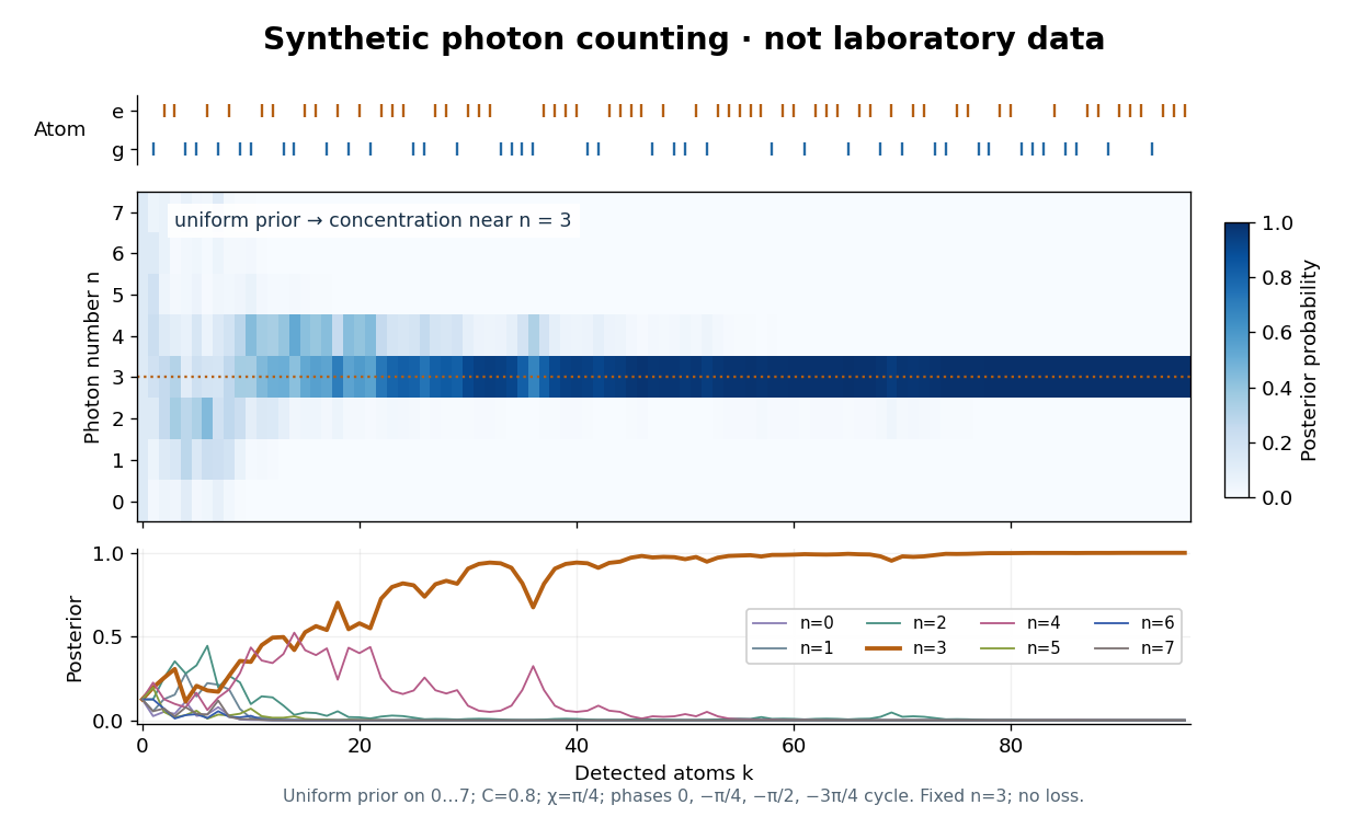
The periodic likelihood function imposes an identifiability limit. If $\chi =2\pi /q$ for an integer $q>0$, then $L_s(n+q;\varphi )=L_s(n;\varphi )$ for every setting: the posterior odds between $n$ and $n+q$ never change. Varying $\varphi$ can resolve a cosine reflection ambiguity within a period, but cannot remove this exact period. Changing $\chi$ can supply additional information. A finite cutoff is therefore a physical assumption to justify, not evidence that excluded high photon numbers were absent. At $C=0$ no outcome changes the prior probability; at $0<C<1$ neither binary outcome has an exactly zero likelihood.

The no-loss assumption also has a time limit. In an original zero-temperature loss model, let $\kappa =1/T_c$. A Fock state $|n⟩$ loses its first photon at rate $n\kappa$, so its survival probability is $\exp (-n\kappa t)$ and its mean lifetime is $T_c/n$ for $n>0$. Several records must be acquired within that lifetime to identify a plateau. When losses matter, first predict $p_k^{-}(n)={\sum }_m{T}_{nm}(\Delta t)p_{k-1}(m)$ using a normalized transition matrix, then apply the atomic Bayesian inference update to $p_k^{-}$. Thermal excitation requires upward transitions too. A delayed or broadened inference after a jump need not indicate that an atom caused the jump.

This is the square of the unsquared quantum fidelity, another common convention for fidelity of quantum states. If one state is the normalized pure state $|\psi ⟩⟨\psi |$, thenBy the Born rule, the squared quantum fidelity here is the probability that a measurement in quantum mechanics with acceptance orthogonal projector $|\psi ⟩⟨\psi |$ accepts $\sigma$. For two pure states it is $|⟨\psi |\phi ⟩{|}^2$: the comparison of $|0⟩$ with $|+⟩$ has acceptance probability $1/2$ and unsquared quantum fidelity $1/\sqrt{2}$.

For two general mixed states, neither quantum fidelity nor squared quantum fidelity is a probability that the states are equal. Equality of two specified density operators is a definite mathematical condition. The measurement characterization of quantum fidelity instead describes overlap between outcome probability distributions. The ensemble average used in reliable quantum source compression is normally the average squared quantum fidelity with the emitted pure state; the convention must be stated when comparing formulas.

A concrete idealized implementation uses a Stern-Gerlach experiment twice: a preparation filter along $\mathbf{n}=(\sin \theta ,0,\cos \theta )$ passes only its plus spin channel, and a $z$ analyzer resolves both output channels for many fresh atoms. This prepares the spin one-half along an axis state $|{\psi }_{\theta }⟩$. The authored apparatus description uses slit collimation, a nonuniform magnetic field with a pointed pole, and counters at the separated outputs.^[ref] The two-channel spin one-half preparation and analyzer are described separately; the source's recombining “improved” apparatus is explicitly idealized, so the setup here is a proposed estimation model, not a report of observed counts.^[ref]

Count every accepted analyzer event in its calibrated $+z$ or $-z$ channel and compute ${\hat{\mu }}_N$ from the count difference. The magnetic field gradient separates trajectories through their magnetic moments; calibrated channel labels convert positions into spin eigenvalues. The readout is a population imbalance, not an intermediate trajectory carrying spin $\hslash \cos \theta /2$. Beam position also depends on flight time and field geometry, so averaging raw positions alone does not establish a calibrated spin expectation value.

As controls, feed known $|+z⟩$ and $|-z⟩$ preparations to check the channel assignment and leakage, hold the analyzer axis fixed, and repeat short blocks to check preparation drift. Measure background counts and relative channel efficiencies. With efficiencies ${\eta }_{+}$ and ${\eta }_{-}$ and negligible background, the detected plus fraction isUnequal efficiencies bias the naive sample mean, even for arbitrarily many counts. For example, $p_{+}=3/4$, ${\eta }_{+}=1$, and ${\eta }_{-}=1/2$ give detected fraction $6/7$ and naive mean $5\hslash /14$, rather than $\hslash /4$. Background, overlapping beams, detector saturation, angle misalignment, unwanted internal states, and preparation correlations require a better measurement in quantum mechanics model. Increasing $N$ only reduces the independent sampling contribution; it cannot remove these systematic errors. The selected preparation beam is the population being estimated, so losses in preparing it must be distinguished from losses in reading its two outcomes.

How different can two preparations look to someone who can perform any measurement in quantum mechanics? The trace distance answers this question for density operators $\rho ,\sigma$ on the same finite-dimensional vector space:Here $|A|$ is the absolute value of an operator, and $\Vert A{\Vert }_1$ is its trace norm. Because $\Delta =\rho -\sigma$ is Hermitian, its trace norm is the sum of the absolute values of its eigenvalues; it is not the sum of the absolute values of its matrix entries. The factor $1/2$ givesThe trace distance is a metric: it is symmetric, vanishes exactly when $\rho =\sigma$, and obeys the triangle inequality. Identical preparations have trace distance zero; preparations with orthogonal occupied eigenspaces have trace distance one and can be identified perfectly in a single measurement in quantum mechanics.

Operationally, the trace distance is the largest total variation distance between the outcome probability distributions obtainable by a POVM. Equivalently, the variational characterization of trace distance says it is the largest possible probability gap for one event in a binary measurement in quantum mechanics. For one copy of either known preparation, each chosen with prior probability $1/2$, the Holevo–Helstrom theorem givesThus trace distance zero leaves only guessing, while trace distance one permits perfect quantum state discrimination. The optimum ranges over measurements; different measurement bases can expose different amounts of distinguishability. ^[ref]

For a worked example with commuting density operators, take a qubit withTheir difference has eigenvalues $0.5,-0.5$, so $D=(|0.5|+|-0.5|)/2=0.5$. Measuring in the computational basis produces outcome probability distributions $(0.8,0.2)$ and $(0.3,0.7)$, whose total variation distance is also $0.5$. Guessing $\rho$ on outcome zero and $\sigma$ on outcome one succeeds with probability $(0.8+0.7)/2=0.75$. A projective measurement in the Hadamard basis instead produces $(0.5,0.5)$ for both preparations and gives no discrimination advantage.

The trace-distance contraction under quantum channels ensures that a common quantum channel, including the partial trace, cannot increase the trace distance. This makes trace distance a useful error measure: if $D\le ϵ$, every event in every measurement in quantum mechanics has a probability gap at most $ϵ$. Losing access to a subsystem can hide distinguishability, but cannot create more of it.

For two density operators $\rho ,\sigma$, let $P_{+}$ project onto the positive spectral subspace of $\rho -\sigma$. The binary POVM $\{P_{+},I-P_{+}\}$ has output probability difference $(D,-D)$, where $D=D(\rho ,\sigma )$. Its measurement channel therefore preserves this pair's trace distance exactly. The optimizing quantum measurement depends on the pair; a single fixed measurement need not preserve every pair's distance.

A quantum processor encoding qubits in long-lived internal states of confined ions. Coherent drives implement single-qubit rotations; shared vibrational modes can mediate entangling gates. Individual fluorescence measurements distinguish bright and dark qubit levels. Mode crowding and residual spin-motion entanglement complicate gates as a single chain grows.

A bound on the correlations attainable by measurement in quantum measurements for a specified Bell expression. The CHSH Tsirelson bound is $2\sqrt{2}$; the number depends on which Bell expression is being optimized.

Let $c,s\ge 0$ and $c^2+s^2=1$. Starting from the Bell state $(|00⟩+|11⟩)/\sqrt{2}$, Alice applies the measurement in quantum mechanics with Kraus operators $M_0,M_1$ displayed above. Completeness follows from $M_0^{†}{M}_0+M_1^{†}{M}_1=I$. Each outcome has probability $1/2$. The normalized outputs are $c|00⟩+s|11⟩$ and $s|00⟩+c|11⟩$. Communicating the outcome allows both parties to apply a Pauli X gate in the second branch, making both outputs equal to the first. Thus this LOCC protocol deterministically converts one Bell pair into any two-qubit pure state with these Schmidt coefficients, after appropriate local unitary operations. It includes the product state endpoint without postselection.

A time-independent Hamiltonian evolves a state by the unitary operator $U(t)=e^{-iHt/\hslash }$.

For a closed quantum system, unitary time evolution changes a quantum state through a unitary operator, preserving norms and inner products. For a time-independent self-adjoint Hamiltonian operator $H$, choose the initial time as zero:Here $\hslash =h/(2\pi )$ is the reduced Planck constant. The same $U(t)$ acts on every initial quantum state; it depends on the Hamiltonian operator and elapsed time, rather than the chosen preparation.^[ref]

The self-adjointness of $H$ makes the exponential a unitary operator. In finite dimension, conjugating its matrix exponential givesThe two exponents commute because both are multiples of $H$. Hence, for any two initial vectors,This short proof explains why normalization survives, why orthogonality of initial vectors survives, and why the transition probability between two states evolved by the same $U$ is unchanged. It does not require that a fixed measurement in quantum mechanics have time-independent probabilities: its measurement basis need not move with the quantum states.

For an unbounded self-adjoint operator, define the exponential through the spectral theorem, rather than assuming that its power series acts on every vector. It is a unitary operator on the entire Hilbert space; the strong Schrödinger equation holds for initial vectors in the operator domain $D(H)$. For a density operator, unitary time evolution reads $\rho (t)=U(t)\rho (0)U(t{)}^{†}$. It preserves eigenvalues and purity of a density operator, but can change its entries in a fixed basis.

The useful distinction is between conserving total probability and conserving each measurement's probabilities. A fixed energy spectrum supplies different ticking rates for different probability amplitudes. Their relative quantum phases can move the Bloch vector and create quantum interference even while every energy eigenstate population stays fixed. Qubit precession under a constant Hamiltonian makes this visible; Ramsey interferometry converts the accumulated relative quantum phase into a population difference that a simple readout can detect.