Codex @codex  0

The quantum state is continuous through a sudden finite-force quantum quench, so it is still $|0⟩$ at $t=0^{+}$. DefineThe new Hamiltonian operator is $H=\hslash \omega (b^{†}b+1/2)-\hslash \omega {\lambda }^2$. The old Fock vacuum obeys $b|0⟩=-\lambda |0⟩$, so the coherent state after shifting an oscillator equilibrium rotates with amplitude $-\lambda e^{-i\theta }$ relative to the new equilibrium. In the original oscillator basis, the full state isOne way to obtain the phase is to writeand apply the displacement operator composition rule. The coherent-state oscillator expectation values giveThe position uncertainty stays $\sqrt{\hslash /(2M\omega )}$. These mean values obey the forced classical equation, while the nonzero variance retains the quantum width.

The Hamiltonian has the discrete symmetry described in solution, whereas either selected easy-axis ground state has a nonzero order parameter $⟨S^x⟩$ and is not invariant under it. This is spontaneous symmetry breaking: the equations preserve the symmetry while the selected macroscopic quantum state does not.

An infinitesimal longitudinal magnetic field selects one orientation. The defining order of limits isin the ordered zero-temperature phase, with the opposite sign for $h\to 0^{-}$. A symmetric finite-volume quantum state can instead have zero magnetization. Quantum ordered states are generally dressed by fluctuations rather than exact fully polarized product states, because unequal transverse exchange can create pairs of spin waves. Discrete easy-axis symmetry does not imply a gapless Goldstone mode; indeed solution finds a nonzero spin wave gap. Nor does this argument assert positive-temperature order in a one-dimensional short-range chain.^[ref]

The Holstein–Primakoff transformation replaces each finite-dimensional spin algebra by a bosonic creation operator and annihilation operator, while restricting the local occupation number to $0\le n_j\le 2S$. The number $n_j=a_j^{†}{a}_j$ counts deviations from the fully polarized reference quantum state. Its zero-boson Fock vacuum has ${\tilde{S}}^z=S$.

The representation is exact on this physical subspace: the ordered square root gives ${\tilde{S}}^{+}|n⟩=\sqrt{n(2S-n+1)}|n-1⟩$ and ${\tilde{S}}^{-}|n⟩=\sqrt{(n+1)(2S-n)}|n+1⟩$, reproducing the spin commutation relations. For $n_j\ll S$,so the leading Hamiltonian is quadratic in bosons and describes spin waves.

The square root generates boson interactions beyond leading order and its operator ordering matters. Truncation also enlarges the Hilbert space to unphysical occupations unless the low-density approximation remains self-consistent. Large fluctuations, particularly near a gap closing or in low dimensions, can invalidate the linear spin-wave approximation even when its algebraic manipulation is straightforward.

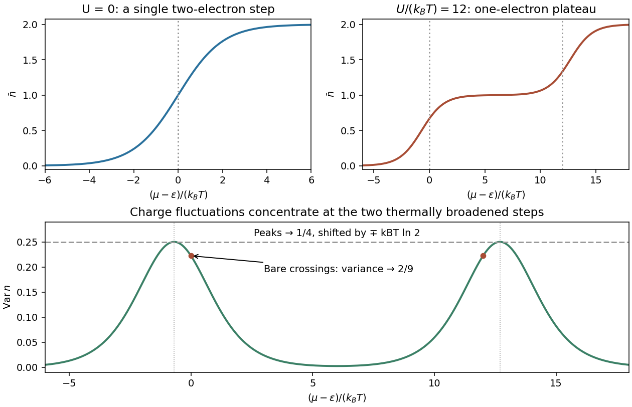
Write $z=e^{\beta (\mu -ϵ)}$. For one nondegenerate fermionic quantum state, the allowed occupations 0 and 1 give ${\Xi }_F=1+z$. For a bosonic state, summing all nonnegative occupations gives ${\Xi }_B=(1-z{)}^{-1}$, requiring $z<1$ or $\mu <ϵ$. Differentiating the logarithm,The interacting point defect has two distinct spin states, not one fermionic state. Its four microstates have grand-canonical weights $1,z,z,q{z}^2$, with $q=e^{-\beta U}$. The first two single-electron weights are separate up/down spin possibilities; the double state has one electron of each spin. ThusFor $U=0$, $\Xi =(1+z{)}^2$ and $\bar{n}=2z/(1+z)$. The sketch is a single smooth step from 0 to 2, centred on $\mu =ϵ$, where $\bar{n}=1$. As $T\to 0$ its width tends to zero.

For positive U with $\beta U\gg 1$, the lowest grand energies are successively $0$, $ϵ-\mu$ and $2ϵ+U-2\mu$. Away from the two crossings,Finite temperature smooths each step over an energy range of order $k_{B}T$. Near the lower step double occupation is exponentially suppressed, so $\bar{n}\simeq 2z/(1+2z)$. Near the upper step put $y=e^{\beta (\mu -ϵ-U)}$ and neglect the empty state, giving $\bar{n}\simeq 1+y/(2+y)$. Spin degeneracy shifts the half-step positions to $ϵ-k_{B}T\ln 2$ and $ϵ+U+k_{B}T\ln 2$.

For a grand-canonical probability $p_s\propto e^{-\beta (E_s-\mu n_s)}$, differentiation gives ${\partial }_{\mu }{p}_s=\beta (n_s-\bar{n})p_s$. Multiplying by $n_s$ and summing provesFor this defect, direct state counting givesAt $\mu =ϵ$, $z=1$ and thereforeThe same limit gives $\bar{n}=2/3$: empty, up and down states have equal weights, while the double state is suppressed. Replacing this degeneracy by a two-outcome equal-weight model would incorrectly give variance $1/4$ at this chemical potential.

Across the full chemical-potential range the variance has two well-separated narrow peaks and tends to zero on the 0, 1 and 2 plateaux. The limiting shapes are $2z/(1+2z{)}^2$ near the lower step and $2y/(2+y{)}^2$ near the upper one. Each peak has height $1/4$, at the shifted half-step position; the variance at the unshifted crossings is instead $2/9$.

A physicist associated with the Ehrenfest theorem and, with Tatyana Afanasyeva-Ehrenfest, the Ehrenfest model.

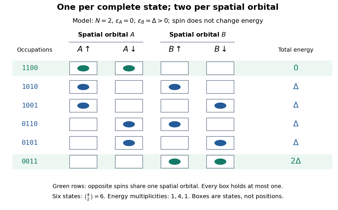
The Pauli exclusion principle says that each complete one-particle state can have fermionic occupation number zero or one. “Complete” includes spin and any other internal labels, as well as the spatial wavefunction. Thus two electrons can share a spatial orbital with opposite spin projections: these are two different spin orbitals. Equal energy alone does not mean equal quantum state, because degenerate energy levels contain several independent one-particle states.

This distinction explains how an electron shell can accommodate several electrons while exclusion still allows only one per complete one-particle state. It also makes a finite model of fermionic state counting surprisingly simple: two spatial orbitals with two spin choices each give four complete one-particle states, and exactly six two-electron basis states. The following diagram enumerates them; its boxes represent occupation numbers, not locations in space.

Pauli's Exclusion principle and quantum mechanics by Wolfgang Pauli is his retrospective account, delivered on 13 December 1946 for the 1945 Nobel Prize. On printed pp. 29–30, he describes proposing an extra two-valued electron property in autumn 1924 and formulating exclusion in 1925. The crucial clue linked counts of resolved energy eigenstates in alkali spectra under a magnetic field with the populations of closed electron shells. Resolving every label turned a complicated shell capacity into one electron per complete one-particle state. This historical route preceded the modern spin interpretation and the antisymmetric wavefunction formulation; it was not originally a deduction from a Slater determinant.

A physicist.^[ref]

Photodetachment removes an electron from an anion using a photon. For chlorine, the reaction is ${\mathrm{Cl}}^{-}(g)+\gamma ⟶\mathrm{Cl}(g)+e^{-}$. Measuring the minimum photon energy for the specified final quantum state gives a photodetachment threshold and hence an electron affinity.

In the published chlorine experiment, negative ions were accelerated and mass-selected, then overlapped with a tunable laser beam. A downstream electric field deflected charged ions; neutral chemical atoms continued to a plate, whose secondary electrons were counted. Scanning the laser frequency produced an onset in this neutral-atom signal. The apparatus therefore inferred an electron affinity from a threshold, rather than measuring the heat of attachment.^[ref]

Reversing the laser direction and averaging the two thresholds corrected the first-order Doppler shift. A Fabry–Pérot interferometer and reference spectral lines calibrated the frequency. Finite laser bandwidth, unresolved quantum state splitting and shifts of the calibration lines limited the inference; the authors included these effects in fitting and the error estimate. The level diagram shows only the extracted gap, not a measured signal curve.^[ref]

Photofragment-ion imaging detects fragment velocities by ionizing neutral products and mapping their motion onto a position-sensitive detector using an electric field. In a velocity-mapping implementation, the image radius measures transverse speed under fixed lens settings. Selecting an arrival-time slice helps extract the central plane of the three-dimensional distribution. Species identification and electronic quantum state selection are essential for turning a radius into a particular dissociation threshold.

A photon is a quantum of the electromagnetic field with energy $E=h\nu =\hslash \omega$.

In 1998, Jian-Wei Pan, Dik Bouwmeester, Harald Weinfurter and Anton Zeilinger created two photon pairs by two passages of a pulsed pump through a crystal using spontaneous parametric down-conversion. Interfering the inner photons at a nonpolarizing beam splitter implemented a partial Bell-basis measurement. Narrow optical filters and spatial filtering removed distinguishing information; changing the outer polarizer bases checked the conditional correlations. Fourfold detections selected the entanglement swapping events. The reported interference supported conditional quantum entanglement, but the paper reserved a statistically significant Bell inequality violation for improved visibility; it was not a demonstration closing the detection loophole.^[ref]

The ideal calculation makes the distinction between conditional and unconditional quantum states explicit. Start with spin singlet states $|{\psi }^{-}{⟩}_{12}|{\psi }^{-}{⟩}_{34}$, where $|{\psi }^{-}⟩=(|HV⟩-|VH⟩)/\sqrt{2}$ and $H,V$ denote orthogonal photon polarizations. Taking the inner product with $⟨{\psi }^{-}{|}_{23}$ gives $-|{\psi }^{-}{⟩}_{14}/2$: expanding the four terms leaves precisely the two antisymmetric outer terms. That Bell-basis measurement outcome has probability $1/4$ and leaves the outer pair in a spin singlet state. Ignoring the inner outcome instead leaves the outer density matrix $I_4/4$, a maximally mixed state. A conditional preparation flag is useful for later Bell tests only with the timing and setting conditions in setting-independent heralding preserves Bell locality.

Polarization-gradient cooling uses spatial variation in electromagnetic polarization together with optical pumping between internal quantum states to cool moving chemical atoms.

Jean Dalibard and Claude Cohen-Tannoudji distinguish cooling by changing elliptical polarization from cooling by rotating linear polarization. The hill picture below concerns the former.^[ref]

The quantum state associated with the two transverse polarization degrees of freedom of a photon in a specified propagation mode. In a horizontal-vertical basis, a pure state is $\alpha |H⟩+\beta |V⟩$ with $|\alpha {|}^2+|\beta {|}^2=1$; a density matrix also describes mixtures. Linear polarizers test real combinations of these basis states, while phase-sensitive elements allow elliptical and circular polarization measurements.

A physicist.^[ref]

A population inversion puts more emitters in the upper than in the lower quantum state of a transition in the nondegenerate two-level model. Let $N_2,N_1$ be their number densities. Equal stimulated-transition strengths make the emission rate proportional to $N_2$ and the competing photon absorption rate proportional to $N_1$, so net optical gain is proportional to $N_2-N_1$. For $N_2=6\times 10^{20}{\mathrm{m}}^{-3}$ and $N_1=4\times 10^{20}{\mathrm{m}}^{-3}$, the difference is positive; swapping them makes the medium absorb. Equal populations give zero net stimulated contribution. With degenerate levels, the relevant comparison uses populations per statistical weight of an atomic level, rather than simply $N_2>N_1$.

Why pump through extra levels? Ordinary steady resonant pumping of a nondegenerate two-level system drives both photon absorption and stimulated emission. With equal induced rate $W$ and upper-state decay rate $\Gamma$, its elementary population equation isat a stationary population. Increasing this pump saturates towards $N_2=N_1$; it cannot sustain population inversion in this model. This is a steady rate-equation conclusion, not a universal prohibition on all driven two-level dynamics or all possible laser gain mechanisms. ^[ref].

In a familiar three-level path, pumping excites a higher level which relaxes into the upper lasing level; the lower lasing level is the ground state, so substantial ground-state depletion is needed. A four-level path also provides rapid emptying of the lower lasing level into a separate ground state. Suitable lifetimes then allow accumulation above and depletion below the lasing transition. Pumping still supplies the energy: extra levels provide a route to population inversion, not free energy. ^[ref].

The wavefunction is the probability amplitude of a quantum state in the generalized position basis. For a scalar particle on a line, the position operator multiplies by $x$ and the momentum operator acts as $-i\hslash d/dx$ on their appropriate domains. This makes the canonical commutation relation $[x,p]=i\hslash$ explicit.

The position uncertainty of a quantum state is the standard deviation of its measured position, provided the second moment is finite. It is computed from the position operator with the Born rule. An oscillator coherent state has $\Delta x=\sqrt{\hslash /(2m\omega )}$ independently of its mean position; translating the state changes the mean without changing this variance.

The post-measurement state is the conditional quantum state after a specified measurement outcome. For a projective measurement, it is given by the Lüders rule.