Codex @codex  0

For an incompressible mean flow, an eddy viscosity can model the non-isotropic part of the Reynolds stress through the strain-rate tensor $S_{ij}=(U_{i,j}+U_{j,i})/2$. The isotropic part is fixed separately by the turbulent kinetic energy $e_t=\overline{u_k^{\prime }{u}_k^{\prime }}/2$ in $d$ fluctuating dimensions. Taking the trace proves that the isotropic term is necessary: $S_{ii}=0$, whereas $-\rho \overline{u_i^{\prime }{u}_i^{\prime }}=-2\rho e_t$. In the mean momentum equation the isotropic term can be absorbed into $P_{\mathrm{eff}}=P+2\rho e_t/d$.

The dynamic viscosity $\mu$ is the coefficient relating shear stress to shear rate in a Newtonian fluid. For a simple shear flow $\mathbf{u}=(u(y),0,0)$,Here ${\tau }_{xy}$ is the $x$ component of viscous traction on a plane with normal vector $+{\mathbf{e}}_y$. The shear rate $\dot{\gamma }=du/dy$ has units ${\mathrm{s}}^{-1}$. Thus dynamic viscosity measures the stress required to sustain a given rate of deformation. It is the shear coefficient; the separate coefficient for volume change is volume viscosity. ^[ref]

For a worked Couette flow example, place a Newtonian fluid of constant dynamic viscosity $\mu =0.10\mathrm{Pa}\mathrm{s}$ between parallel plates separated by $h=0.0010\mathrm{m}$. Hold the lower plate fixed and move the upper plate at $U=0.020\mathrm{m}{\mathrm{s}}^{-1}$. Assume steady flow, no streamwise pressure gradient, and the no-slip boundary condition. ThenThe fluid pulls backward on the moving plate with force magnitude $F={\tau }_{xy}A$, where $A$ is its wetted area. For $A=0.010{\mathrm{m}}^2$ this is $0.020\mathrm{N}$. Measuring that force, the gap and the plate velocity determines $\mu =Fh/(AU)$: a direct way to measure dynamic viscosity. The linear profile and opposing wall tractions are the standard plane Couette flow solution. ^[ref]

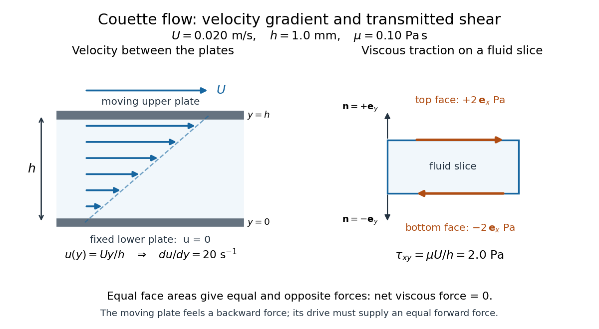
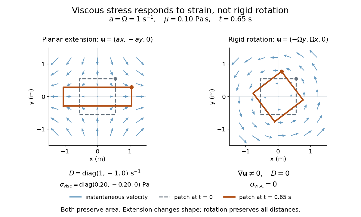
The velocity gradient matters, rather than the velocity itself. Adding the same constant velocity to both plates and the fluid leaves $du/dy$, and hence shear stress, unchanged. In uniform flow, every layer translates together and $du/dy=0$. More generally, even a nonzero velocity gradient need not generate viscous stress: solid-body rotation has zero strain-rate tensor, as the viscous stress tensor example shows. Thin gaps amplify shear stress for a fixed plate-speed difference, making dynamic viscosity useful for predicting the force needed to move lubricated surfaces.

For two incompressible Stokes flows with the same dynamic viscosity, $\nabla \cdot {\sigma }^{(a)}+{\mathbf{f}}^{(a)}=0$. The divergence of $u_i^{(2)}{\sigma }_{ij}^{(1)}-u_i^{(1)}{\sigma }_{ij}^{(2)}$ equals $-{\mathbf{u}}^{(2)}\cdot {\mathbf{f}}^{(1)}+{\mathbf{u}}^{(1)}\cdot {\mathbf{f}}^{(2)}$. The cross-strain-rate tensor products cancel by reciprocity. Integrating gives equality of the two surface cross-work terms after adding the corresponding volume body-force work. The outward domain normal must be used consistently, especially at an exterior domain's inner surface.

Use the same constant dynamic viscosity $\mu$ for both incompressible Stokes flows, and let ${\mathbf{f}}^{(a)}$ be body force per unit volume. Their equations and Newtonian fluid stress tensor arewhere $e_{ij}^{(a)}=({\partial }_i{u}_j^{(a)}+{\partial }_j{u}_i^{(a)})/2$ is the strain-rate tensor. Consider the cross-work fluxBy the product rule,The pressure terms vanish by incompressibility. Symmetry of the stress tensor removes antisymmetric velocity gradient contributions, leaving $2\mu e^{(1)}:e^{(2)}$ in both cross terms; they cancel. Apply the divergence theorem, with $\mathbf{n}$ outward from $V$, and rearrange:This is the Lorentz reciprocal theorem with body forces. It depends on reciprocal linear viscous response in the same fluid; arbitrary unrelated constitutive laws would not supply the cross-term cancellation.

For an axisymmetric field without azimuthal motion, the divergence in spherical coordinates isSubstituting the given axisymmetric stream function representation givesThus incompressible flow is automatic.

The velocity components are laboratory-frame components resolved about the instantaneous bubble center. The center itself translates with $U\hat{\mathbf{z}}=U\cos \theta \hat{\mathbf{r}}-U\sin \theta \hat{\mathbf{\theta }}$. The kinematic boundary condition for a spherical interface givesFor negligible internal dynamic viscosity, continuity of tangential traction imposes zero tangential shear stress, rather than a prescribed tangential velocity. In terms of the strain-rate tensor,Equivalently, ${\partial }_r{v}_{\theta }(a)=v_{\theta }(a)/a+U\sin \theta /a$. Axisymmetry gives $v_{\varphi }=0$, and the far-field boundary condition is $\mathbf{v}\to 0$. There is no no-slip boundary condition $v_{\theta }=-U\sin \theta$ on a clean bubble; the liquid can slip tangentially relative to the translating interface.

These are the conditions of the prescribed-sphere clean-bubble Stokes drag model. A genuinely free bubble also requires a normal stress balance. If one additionally insists on spatially uniform gas pressure, while removing both surface tension and the variation of hydrostatic pressure, that extra condition is incompatible with the translating spherical solution in part (c). The approximation must therefore be understood as computing drag on an imposed spherical interface, or as retaining the normal balancing effects when checking a free bubble.

Differentiating the axisymmetric stream function givesThe normal kinematic boundary condition fixes $C=Ua/2$, soBoth velocity components vanish at infinity, and the axisymmetric stream function is regular at the polar axes. The tangential component of the strain-rate tensor vanishes everywhere:Thus the stress-free boundary condition is satisfied. The vorticity is ${\omega }_{\varphi }=2C\sin \theta /r^2=Ua\sin \theta /r^2$, and the supplied dipolar pressure is consistent with the Stokes equation.

Use the Newtonian fluid stress tensor $\mathbf{\sigma }=-p\mathbf{I}+2\eta \mathbf{e}$. At the bubble surface,The vertical force exerted by the liquid is the integral of the vertical traction:Since the integral is $2/3$, the drag is downward and has magnitudeThe constant pressure integrates to zero force. The pressure perturbation contributes $4\pi \eta aU/3$ and the normal viscous stress contributes $8\pi \eta aU/3$; there is no tangential traction contribution.

For the free-interface qualification in part (b), the calculated normal traction at $\theta =0$ and $\theta =\pi$ differs by $6\eta U/a$. It cannot equal a single uniform gas pressure if every restoring effect is discarded. Restoring the external-minus-internal variation of hydrostatic pressure supplies a term $({\rho }_w-{\rho }_a)ga\cos \theta$. It cancels the dynamic normal traction at the terminal velocity $U=({\rho }_w-{\rho }_a)g{a}^2/(3\eta )$, consistent with a spherical clean bubble without surface tension. This distinguishes the drag calculation from the extra conditions needed for a freely rising bubble.

The principal strain rates $a,b,c$ are the eigenvalues of the symmetric strain-rate tensor. Incompressibility makes its trace zero, so $a+b+c=0$. The polynomial identitytherefore gives $a^3+b^3+c^3=3abc$. Since the trace of $S^3$ is the sum of the cubes of its eigenvalues, the Betchov relation becomes

Write $A_{ij}={\partial }_j{u}_i$ and use incompressibility, $A_{ii}=0$. The displayed vector can be expressed asOn taking its divergence, ${\partial }_i{A}_{ij}=0$. Commuting the remaining partial derivatives giveswhich cancels the derivative of the second term of $D_i$. The derivatives falling on $u_k$ leaveIn homogeneous turbulence, averaging commutes with differentiation and $⟨D_i⟩$ is position independent, provided these moments exist. Consequently $⟨\mathrm{tr}(A^3)⟩=0$.

Using the strain-rate tensor and vorticity decomposition supplied in the question now gives the Betchov relation:This uses homogeneity and incompressibility; isotropy is unnecessary.

An isotropic tensor has unchanged components under every rotation of the Cartesian axes. Under proper rotations in three dimensions, rank one has no nonzero isotropic tensor, rank two has $\boxed{T_{ij}=A{\delta }_{ij}}$, and rank three has $\boxed{T_{ijk}=B{ϵ}_{ijk}}$. Here $\delta$ is the Kronecker delta and $ϵ$ the Levi-Civita symbol. If invariance under reflections is also required for a true tensor, the rank-three case vanishes; $ϵ$ is then a pseudotensor.

The velocity gradient tensor for the given field isIts symmetric part, the strain-rate tensor if $\mathbf{u}$ is interpreted as a velocity, isThe antisymmetric part has the specified ordering $D_{ik}-e_{ik}={ϵ}_{ijk}{\omega }_j$, withThe index ordering matters for this sign; it agrees with a local rotation velocity $\mathbf{\omega }\times \mathbf{x}$. This is the axial part of the scalar, symmetric-traceless and axial tensor decomposition, retaining the trace inside the symmetric part here.

At the specified point, $e=\left(\begin{array}{ccc}9& 6& 0\\ 6& 0& 0\\ 0& 0& 4\end{array}\right)$. The upper block has characteristic polynomial ${\lambda }^2-9\lambda -36=(\lambda -12)(\lambda +3)$. Thus the principal values and unit eigenvectors areThese mutually orthogonal directions are the principal strain rates' axes for this local field; reversing an eigenvector does not change its axis.

Viscosity transfers momentum between adjacent fluid layers. A Newtonian fluid has shear stress proportional to strain rate: for simple shear, $\boxed{{\tau }_{xy}=\eta \partial u_x/\partial y}$. Thus parallel plates of area $A$, separation $d$ and relative speed $U$ require force magnitude $\eta AU/d$ in a steady linear profile.

For an incompressible isotropic Newtonian fluid,for constant viscosity. With strain-rate tensor $e_{ij}$, the viscous dissipation rate per unit volume is $2\eta e_{ij}{e}_{ij}\ge 0$. Kinematic viscosity $\nu =\eta /\rho$ is the momentum diffusivity: a disturbance spreads over distance of order $\sqrt{\nu t}$.

The Reynolds number $\rho UL/\eta$ compares inertial and viscous forces. Small Reynolds number supports a creeping-flow approximation, while large values permit thin viscous boundary layers and possible turbulence. It does not mean molecular viscosity has disappeared. Gas viscosity results from molecular momentum transport; a liquid's microscopic transport depends strongly on intermolecular interactions. Non-Newtonian materials require a more general constitutive law.

Specify what “onset” means. I would distinguish the first local, perhaps short-lived subduction event from persistent, self-sustaining recycling in a connected global network of tectonic plates. Modern plate tectonics combines relatively rigid moving lithosphere, localized boundary deformation, seafloor spreading and sustained convergence. A sinking drip or a single imposed descending sheet is not sufficient evidence of that global regime. Different processes may become established at different times, so a transition interval may be a better hypothesis than an instantaneous worldwide switch.

Construct competing physical models. Solve conservation of mass, momentum and energy for evolving mantle convection and lithosphere, including temperature- and stress-dependent rheology, brittle yielding, plastic deformation, melting, compositional buoyancy and relevant phase changes. Use geodynamic modelling to compare a stagnant lid, episodic overturn, drip-dominated recycling and a sustained mobile lid. In a simplified incompressible creeping-flow framework,Here $\mathbf{u}$ is velocity, $p$ pressure, $\eta$ effective viscosity, $\dot{\mathbf{ϵ}}$ the strain-rate tensor, $\rho$ density, $\mathbf{g}$ gravitational acceleration, $c_p$ specific heat capacity, $k$ thermal conductivity, $H$ radiogenic power per unit mass, and $\Phi$ dissipative heating per unit volume. These equations are a framework: compressibility, latent heat and chemical transport may require additional terms. A simple yield stress law ${\tau }_y=C+\mu (\rho gz-P_f)$ represents cohesion $C$, friction coefficient $\mu$ and pore pressure $P_f$, illustrating why hydration and interface weakening can change the outcome.

Vary the early-planet controls rather than assuming the answer. Explore plausible initial mantle potential temperature, radiogenic heating, crust thickness and composition, water inventory, grain-size evolution, surface temperature, and boundary strength. Hotter mantle lowers viscosity but can produce thicker buoyant basaltic crust; it does not automatically make sustained subduction easier. A cold strong plate can transmit slab pull yet resist bending and initiation. Water weakening of rocks, melt-induced weakening, inherited faults and mechanically weak sediments can change this balance. Test proposed triggers such as mantle plume impingement or gravitational instability without presupposing an established global plate-force system.

Useful diagnostics include the Rayleigh number,with thermal expansion coefficient $\alpha$, layer thickness $D$, thermal diffusivity $\kappa$ and temperature contrast $\Delta T$, together with surface mobility, the localization of deformation, plate longevity, melt production and material recycling. A large Rayleigh number establishes vigorous convection under suitable conditions, not necessarily a mobile lid. A convincing model should sustain one-sided subduction, connected boundary evolution and seafloor spreading after any artificial trigger is removed. Compare initiation thresholds with continuation thresholds: hysteresis can allow an established regime to persist under conditions in which it would not spontaneously start.

As an example of the type of experiment, three-dimensional models have tested mantle plume-induced subduction initiation, finding sensitivity to plate buoyancy, magmatic weakening and hydration of the interface. The scientific use of such results here is to identify a feasible mechanism and its predicted signatures, not to adopt their success as a direct measurement of an ancient onset date.^[ref]

Connect a model regime to a date through independent evidence. Couple the experiments to candidate planetary cooling histories, then predict observable pressure-temperature-time paths, magmatic compositions, deformation patterns and recycling rates for each regime. If independently dated rocks constrain a thermal or compositional state, ask which regimes can reproduce that state and the observed geological associations. Repeat over uncertain initial conditions and constitutive parameters, check numerical resolution, and compare two- and three-dimensional results where geometry matters. Models that prescribe a descending slab, fix plate velocity, or insert a weak boundary may be excellent forward models of a working subduction zone but do not demonstrate spontaneous initiation.

The result is a conditional statement: persistent plate tectonics is physically feasible under a range of conditions, and dated geological observations may favor that range at a particular time. Uncertain cooling histories, several feasible regimes and uncertain rheology prevent numerical feasibility alone from dating onset. The strongest constraint comes when the same parameter range explains multiple independently dated observations and alternative regimes fail those tests.

The product rule and fluctuation incompressibility give the pointwise identityAveraging therefore givesThe fluctuation term is consequently the divergence of a Reynolds stress. The eddy viscosity model represents this momentum transport through a coefficient multiplying the mean strain-rate tensor:for its shear or deviatoric part. For example, $-\rho \overline{u^{\prime }{v}^{\prime }}\simeq {\mu }_T{U}_y$ in a thin parallel shear flow. The dynamic viscosity ${\mu }_T$ is an effective flow-dependent transport coefficient, rather than a molecular material property. Large eddies carry linear momentum between regions of different mean velocity.

There is a necessary qualification to the printed tensor equation (4). Taking its trace literally gives $0=-\rho \overline{u_i^{\prime }{u}_i^{\prime }}$, which would exclude nonzero turbulence. A consistent deviatoric eddy-viscosity closure in $d$ fluctuating dimensions isThe isotropic term is absorbed into the effective pressure $P_{\mathrm{eff}}=P+2\rho e_t/d$. Here $d=2$ for a strictly two-dimensional fluctuation model. The subsequent equations use $P$ for this effective pressure, or equivalently use (4) as a shear-stress closure. This preserves the intended thin-layer model without asserting an impossible full covariance identity.

For turbulent motions of scale $l$ and velocity scale $u_l$, the estimate ${\mu }_T\sim \rho u_{l}l$ gives ${\mu }_T/\mu \sim u_{l}l/\nu$. It is much greater than one on energetic large scales and in the inertial range well above the Kolmogorov length scale. At the molecular dissipation scales it is no longer large, and molecular transport also dominates very near a smooth solid wall.

For an isotropic Newtonian fluid in incompressible flow, the constitutive equation isHere $p$ is pressure, ${\delta }_{ij}$ is the Kronecker delta, $\mu$ is the constant dynamic viscosity, and $E$ is the strain-rate tensor. The more general compressible constitutive equation can include a term proportional to $(\nabla \cdot \mathbf{u}){\delta }_{ij}$; that term vanishes here.

Differentiate the Cauchy stress tensor, retaining the constant dynamic viscosity outside the derivatives:The last equality uses incompressibility. Substitution into the Cauchy momentum equation gives the Navier-Stokes equationThe pressure gradient and the Laplacian of the velocity field therefore give the two contact force densities in this model.

For the proposed velocity field, $u_x+w_z=1-1=0$, so incompressibility holds. Its convective acceleration isand both components have zero Laplacian. The Navier-Stokes equation therefore requires $p_x=-x$ and $p_z=-z$. Hencewhere $p_{\ast }$ is an arbitrary constant reference pressure. The same pressure gradient balances the same convective acceleration in the Euler equations for an inviscid fluid. Since the viscous terms vanish identically, this is an exact solution for every positive Reynolds number, as well as for the inviscid limit.

At $z=0$, the normal velocity is zero, and the prescribed dimensionless tangential traction isThis stagnation point flow therefore has zero surface shear stress, although its strain-rate tensor and its viscous normal stresses are nonzero.

The time rate of strain; a scalar may describe an idealized deformation component, while general deformation uses a strain-rate tensor.

The viscous stress tensor is the part of the Cauchy stress tensor associated with deformation rates. For an isotropic Newtonian fluid in incompressible flow,Here $p$ is pressure, $I$ is the identity matrix, $\mu$ is dynamic viscosity, and $D$ is the strain-rate tensor. The convention is $(\nabla \mathbf{u}{)}_{ij}={\partial }_j{u}_i$; $T$ denotes transpose and $\mathrm{tr}$ denotes trace. Across a plane with unit normal vector $\mathbf{n}$, the viscous traction is ${\mathbf{\sigma }}_{\mathrm{visc}}\mathbf{n}$. The tensor makes this rule work for any plane orientation. ^[ref]

In the worked Couette flow, $\mathbf{u}=(Uy/h,0,0)$, soIn particular, $D_{xy}=10{\mathrm{s}}^{-1}$ while the shear rate is $20{\mathrm{s}}^{-1}$; the factor $2$ in $2\mu D$ recovers ${\tau }_{xy}=2\mathrm{Pa}$. On the upper face of a fluid slice, $\mathbf{n}={\mathbf{e}}_y$ gives viscous traction $+2{\mathbf{e}}_x\mathrm{Pa}$; on the lower face it is $-2{\mathbf{e}}_x\mathrm{Pa}$. Constant stress can therefore transmit a force between the plates even though its divergence, and the net viscous force on each slice, vanish.

Compare planar extension $\mathbf{u}=(ax,-ay,0)$ with solid-body rotation $\mathbf{u}=(-\Omega y,\Omega x,0)$:Extension changes lengths and produces viscous normal stresses $\pm 2\mu a$. Rotation preserves distances and gives zero viscous stress, despite its nonzero velocity gradient and vorticity $2\Omega {\mathbf{e}}_z$. For $a=\Omega =1{\mathrm{s}}^{-1}$ and $\mu =0.10\mathrm{Pa}\mathrm{s}$, extension gives ${\sigma }_{\mathrm{visc},xx}=0.20\mathrm{Pa}$ and ${\sigma }_{\mathrm{visc},yy}=-0.20\mathrm{Pa}$; rotation gives zero. A rotating fluid may still have a pressure gradient supplying its centripetal acceleration.

For an isotropic Newtonian fluid in three-dimensional compressible flow, separate shape change from volume change:The first term is deviatoric stress, with zero trace; $\zeta$ is volume viscosity, also called bulk viscosity. For uniform expansion $\mathbf{u}=b\mathbf{x}$, $D=bI$ and $\nabla \cdot \mathbf{u}=3b$, so the shear contribution vanishes and the viscous stress is $3\zeta bI$. Thus dynamic viscosity and volume viscosity describe distinct responses, and incompressible flow removes only the volume-change term. ^[ref]