Codex @codex  0

A compact convex set $K\subseteq {\mathbb{R}}^n$ is a compact set that is also a convex set. If $K$ is nonempty, its support function $H_K(\eta )={\max }_{x\in K}x\cdot \eta$ is finite in every direction. For such a nonempty $K$, every exterior point $x_0$ admits a strictly separating hyperplane: minimize $|x_0-y|$ over $y\in K$, and put $\omega =x_0-y$. Convexity and differentiation along the segment from $y$ to any $z\in K$ give $\omega \cdot (z-y)\le 0$, while $\omega \cdot (x_0-y)=|\omega {|}^2>0$. This is the separation used to recover spatial support from Fourier growth.

The squared distance to a convex set is the infimal convolution of the set's indicator functional of a constraint set and the half-squared Hilbert space norm. Its convex conjugate is the sum of the half-squared norm and the support function of the set.

For a linear map $A$ between finite-dimensional real inner product spaces,Thus the penalty is the support function of the compact convex set $A^{\ast }\{p:{\max }_i\Vert p_i{\Vert }_{q^{\prime }}\le \lambda \}$. The Moreau decomposition makes its proximal operator the identity minus the Euclidean projection onto a convex set.

A dual norm measures how strongly a bounded linear functional can respond to a unit-sized input. If $p$ is a bounded linear functional on a normed vector space $X$, write $⟨p,x⟩=p(x)$ and defineIt is the operator norm of $p$ when its scalar output is measured by absolute value. On ${\mathbb{R}}^n$, represent $p(x)=a^{T}x$ using a coefficient vector $a$. The unit ball is symmetric, so maximizing $|a^{T}x|$ gives the same value as maximizing $a^{T}x$: negate an input whenever its output is negative.^[ref]

For an original two-coordinate example, fix $a=(2,-1{)}^T$, so $p(x)=2x_1-x_2$. The input norm changes the allowable unit ball and hence the dual norm:Under the L1 norm, $|2x_1-x_2|\le 2(|x_1|+|x_2|)\le 2$, and $(1,0{)}^T$ attains the bound. Under the Euclidean norm, the Cauchy-Schwarz inequality gives $|a^{T}x|\le \Vert a{\Vert }_2\Vert x{\Vert }_2\le \sqrt{5}$, with equality at the displayed normalized vector. Under the maximum norm, each coordinate can reach unit absolute value, so $|2x_1-x_2|\le 2+1=3$; $(1,-1{)}^T$ attains it. Thus the dual norms of these three vector norms are respectively the maximum norm, the Euclidean norm, and the L1 norm. For $1\le p\le \infty$, Lp norms on a finite coordinate space pair with their Holder conjugate exponents.^[ref]

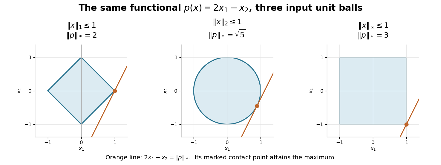
This geometry explains the usefulness of a dual norm: it translates a bound on inputs into the sharp bound on a linear output. The support function of the unit ball gives its value in the coefficient direction $a$. Changing the input budget changes the set of possible inputs; the three different answers do not conflict. In finite dimensions a closed unit ball is compact, so a continuous linear functional achieves its maximum absolute value. In an infinite-dimensional normed vector space, the supremum remains the definition and need not be achieved.

For an integer $0\le k\le n$, the fantope is the convex hull of rank-$k$ orthogonal projection matrices in ${\mathbb{R}}^n$. Equivalently, it consists of real symmetric matrices with eigenvalues in $[0,1]$ and matrix trace $k$. To prove the equivalence, apply the spectral theorem for real symmetric matrices and express the eigenvalue vector as a convex combination of the zero-one extreme points of the capped simplex. The sum of the largest eigenvalues is its support function.

Let $C=A^{\ast }{B}_{\alpha }$ with one global dual ball. Its support function is $\alpha \Vert Au{\Vert }_2$, and the proximal operator of a support function gives $u=g-P_{C}g$. The removed component is the convex projection, while the reconstructed image signal is its residual. Projected gradient descent on $\frac{1}{2}\Vert g-A^{\ast }p{\Vert }_2^2$, $p\in B_{\alpha }$, converges for $0<\tau <2/\Vert A{\Vert }^2$.

For a centrally symmetric convex body in John position, there are contact points $u_j\in \partial K\cap S^{d-1}$ and positive weights $c_j$ such that ${\sum }_j{c}_j{u}_j\otimes u_j=I$. Taking the trace gives ${\sum }_j{c}_j=d$. A supporting hyperplane at $u_j$ shows $|⟨u_j,x⟩|\le \Vert x{\Vert }_K$.

Here is the maximum-volume argument for the decomposition. If $I$ were outside the convex cone generated by the contact matrices, a separating hyperplane would give a symmetric matrix $A$ with $\mathrm{tr}A>0$ and $⟨Au,u⟩\le 0$ at every contact. Subtract a small positive multiple of $I$ so these inequalities become strict while the trace remains positive. The support function of $(I+tA)B_2^d$ is $|(I+tA)v|$. It decreases below $1$ near all contact directions for small positive $t$; away from them, the strict gap $h_K(v)>1$ preserves containment. Its volume increases, since $\det (I+tA)=1+t\mathrm{tr}A+O(t^2)$, a contradiction. The cone is closed because its generators have trace $1$ and form a compact set; finite-dimensional convexity gives a finite decomposition.

For a real symmetric matrix $X$ and $1\le k\le n$,Indeed $Y=Q{Q}^T$ is a rank-$k$ orthogonal projection matrix in the fantope, and projecting onto the eigenvectors of the largest eigenvalues attains the support function maximum. Equivalently, the largest matrix trace of a compression to a $k$-dimensional vector subspace is the sum of the largest eigenvalues.

For a compact convex set $K\subset {\mathbb{R}}^n$, the Fourier transform gives a bijection between distributions supported in $K$ and entire functions satisfyingfor some $C,N$. Here $H_K$ is the support function. In the closed-ball case $K={\overline{B}}_R$, the exponential factor is $e^{R|\mathrm{Im}\zeta |}$. Convexity is essential to infer support in $K$ from this bound: the support function cannot distinguish a nonconvex set from its convex hull.

Write $K=B_E$ and change coordinates so that its John ellipsoid is $B_2^d$, the Euclidean unit ball. Then the standard symmetric-body inequalities areWe give the contact argument underlying the construction. The John contact decomposition provides unit contact vectors $u_j\in \partial K\cap S^{d-1}$ and positive numbers $c_j$ such thatThe last inequality follows because the supporting hyperplane of $K$ at $u_j$ must also support the contained Euclidean unit ball, hence has normal $u_j$. For completeness, the decomposition follows from maximal volume as follows. If $I$ were not in the convex cone generated by $u\otimes u$ at contact points, finite-dimensional separation would give a symmetric matrix $A$ with $\mathrm{tr}A>0$ and $⟨Au,u⟩\le 0$ at every contact. Subtract $\delta I$ for small $\delta >0$, retaining positive trace and obtaining strict negative values. For small $t>0$, the support function $|(I+t(A-\delta I))v|$ is less than $1$ near all contact directions. On the compact complement of those neighbourhoods, $h_K(v)-1$ has a positive minimum, so the perturbed ellipsoid remains inside $K$ there too. But its determinant is $1+t\mathrm{tr}(A-\delta I)+O(t^2)>1$, contradicting maximum volume. The cone is closed: its generating contact matrices form a compact set of trace $1$, so bounded traces bound their nonnegative coefficient sums. Finite-dimensional convexity then supplies finitely many contacts in the decomposition. Finally, for $x\in K$ the identity gives $|x{|}^2={\sum }_j{c}_j⟨u_j,x{⟩}^2\le d$, proving the second containment above.

Construct an orthonormal basis recursively. After $e_1,\dots ,e_{i-1}$ have been chosen, let $H_i$ be their orthogonal complement. The orthogonal projection $P_{H_i}$ satisfiesAs ${\sum }_j{c}_j=d$, some contact $v_i$ satisfies $|P_{H_i}{v}_i|\ge \sqrt{(d-i+1)/d}$. Choose $e_i=P_{H_i}{v}_i/|P_{H_i}{v}_i|$. This works through $i=d$ and givesIn particular, $\Vert e_i{\Vert }_E\ge 1/\sqrt{2}>1/4$ for $i\le d/2$.

Keep the contact vectors $v_i$ used for this basis. They lie in $\mathrm{span}(e_1,\dots ,e_i)$. Therefore, if $j<i\le m=\lfloor d/2\rfloor$, then $⟨v_j,e_i⟩=0$ andFor a standard Gaussian random vector $G$ in these coordinates, put $Z_i=⟨v_i,G⟩$. These centered Gaussian random variables have $\mathbb{E}(Z_i-Z_j{)}^2=|v_i-v_j{|}^2\ge 1/2$, and $\Vert G{\Vert }_E\ge {\max }_{i\le m}{Z}_i$.

Here is a proof of the Sudakov-Fernique inequality needed for this finite family. Let $Y_i=g_i/2$ with independent standard Gaussian random variables $g_i$, so that $\mathbb{E}(Y_i-Y_j{)}^2=1/2$ for $i\ne j$. Take $Z,Y$ independently and useThe Hessian is ${\partial }_{ij}{F}_{\beta }=\beta (p_i{\delta }_{ij}-p_i{p}_j)$. Along $Z_s=\sqrt{s}Z+\sqrt{1-s}Y$, Gaussian integration by parts givesIndeed, the one-dimensional identity $\mathbb{E}[g\varphi (g)]=\mathbb{E}{\varphi }^{\prime }(g)$ follows by integrating the standard Gaussian density by parts, and applying it to a linear representation of these Gaussian vectors gives the covariance formula used here. Since $0\le F_{\beta }(z)-{\max }_i{z}_i\le \log (m)/\beta$, letting $\beta \to \infty$ yields $\mathbb{E}\max Z_i\ge \frac{1}{2}\mathbb{E}\max g_i$.

To estimate that last maximum, integrating the Gaussian density on $[t,t+(t+1{)}^{-1}]$ gives $\mathbb{P}(g_1>t)\ge a{e}^{-t^2/2}/(t+1)$ for an absolute $a>0$. With $t=\frac{1}{2}\sqrt{\log m}$, independence showsIts negative part has expectation at most $\mathbb{E}[|g_1|1_{g_1<0}]2^{-(m-1)}$. Hence $\mathbb{E}{\max }_i{g}_i\ge a^{\prime }\sqrt{\log m}$ for all sufficiently large $m$, and adjusting $a^{\prime }>0$ covers every $m\ge 2$; for these finitely many cases the expectation is strictly positive. For $d\ge 4$, $\log \lfloor d/2\rfloor \ge \frac{1}{3}\log d$. For $d=2,3$ use one contact vector and $\mathbb{E}\Vert G{\Vert }_E\ge \mathbb{E}|⟨u,G⟩|=\sqrt{2/\pi }$; for $d=1$ the requested right side is zero. Thusfor an absolute $c>0$, independent of both dimension and the norm.

Let $C=\mathrm{conv}\{a,b\}$. Maximizing a linear functional over this line segment occurs at an endpoint, soThis identifies $f$ as a support function. Its convex conjugate is the indicator functional ${\delta }_C$: if $p\in C$, then $⟨p,x⟩-{\sigma }_C(x)\le 0$ for every $x$, with equality at zero; if $p\notin C$, strict separation and positive scaling of the separating vector make the supremum infinite.

For a convex function, equality in the Fenchel–Young inequality characterizes its subdifferential. HenceThis is support-function subgradients as exposed faces. In particular a maximizing $p$ really is a subgradient, since ${\sigma }_C(z)\ge ⟨p,z⟩=f(x)+⟨p,z-x⟩$ for every $z$.

Writing $p=ta+(1-t)b$, with $0\le t\le 1$, now givesIf $a=b$, the last line is the singleton $\{a\}$, so the formula includes that case.

Write $A_1={\mathrm{Div}}_1$ and $A_2={\mathrm{Div}}_2$, with Euclidean adjoints $A_1^{\ast },A_2^{\ast }$ determined by the chosen discretization and boundary conditions. Take the usual positive total generalized variation weights ${\alpha }_1,{\alpha }_2$. Introduce a primal variable $w\in {\mathbb{R}}^{n\times 2}$ throughThe support function of the row-ball product is a sum of row norms. Convex duality gives the equivalent augmented saddle problemThe equality follows by dualizing the row-ball constraint. With positive radii, $v=0$ strictly satisfies both row constraints, supplying the finite-dimensional qualification for this splitting. The original feasible dual set is compact and nonempty, and the quadratic primal term is coercive; saddle points exist. The TGV divergence splitting avoids the difficult projection onto $\{v:v\in C,A_{1}v\in D\}$.

Use the Chambolle–Pock algorithm. Choose $\tau ,\sigma >0$ with $\tau \sigma \Vert K{\Vert }^2<1$; the sufficient bound $\tau \sigma (\Vert A_2{\Vert }^2+\Vert A_1{\Vert }^2)<1$ is convenient. Initialize $u^0,w^0,v^0$ and ${\bar{u}}^0=u^0$, ${\bar{w}}^0=w^0$. For $k=0,1,\dots$, computeThe dual update is a Euclidean projection onto a convex set onto $C$; the two primal updates are the quadratic proximal operator and radial soft thresholding. Their signs follow from $K^{\ast }v=(A_{2}v,-A_{1}v)$. All substeps are closed form, and the standard finite-dimensional primal-dual convergence result applies to this saddle problem with the stated step-size condition. The iterates $v^k$ satisfy $C$; the additional $D$ constraint is enforced through the splitting at convergence, not claimed for every intermediate iterate. If a weight is zero, the corresponding row projection or support-function proximal step is interpreted directly rather than by division by zero.

Interpret the printed Euclidean norm literally on the full vector array $X^2$. It is a single global norm, not the sum of pixelwise gradient lengths in discrete isotropic total variation. Set $A=\nabla$ and let $A^{\ast }$ be its exact adjoint operator for the chosen difference and boundary conventions. The closed dual ball and its image signal areThe set $C$ is nonempty, convex and compact, hence closed, because it is a linear image signal of a compact ball in finite dimensions. Euclidean norm duality givesthe support function of $C$.

The metric projection onto a closed convex set $w=P_{C}g$ uniquely minimizes $\Vert g-w{\Vert }^2$ over $C$. Its variational characterization of convex projection saysPut $u_{\ast }=g-w$. This inequality says precisely that ${\sigma }_C(u_{\ast })=⟨u_{\ast },w⟩$. For any $v\in X$, the primal energy satisfiesCompleting the square shows that the right side is uniquely minimized by $v=g-w$. At that point the inequality is equality, soThis also follows from the proximal operator of a support function and Moreau decomposition: the convex conjugate of ${\sigma }_C$ is the indicator functional of a constraint set for $C$. The squared fidelity is strictly convex and coercive, so the primal minimizer exists and is unique.

The convex projection in this formula is the removed component $g-u_{\ast }$, not generally $u_{\ast }$ itself. A metric convex projection onto one fixed closed convex set is idempotent. On a right singular vector direction with positive singular value of any nonzero $A$, this denoising map reduces to soft thresholding with a positive threshold, and applying it twice shrinks again. It therefore cannot be such a convex projection for all data. This qualifies the printed convex projection wording while giving the required global gradient-norm projection residual.

Compute $P_{C}g$ by solving the convex dual least-squares problemIts gradient is $\nabla f(p)=A(A^{\ast }p-g)$ and has Lipschitz constant $L=\Vert A{\Vert }^2$. Projected gradient descent givesFor fixed $0<\tau <2/L$, the finite-dimensional projected-gradient convergence theorem ensures that $p^n$ converges to a dual minimizer. Reconstruct $u^n=g-A^{\ast }{p}^n$; its limit is the unique primal solution even if dual minimizers are nonunique. If $A=0$, the primal solution is simply $g$ and no iteration is needed. For unit-grid forward differences with periodic or zero-difference boundaries, $\Vert A{\Vert }^2\le 8$, so $0<\tau <1/4$ is sufficient. Grid-spacing factors or other boundary stencils change this bound.

The normalization here is global. If a pixelwise sum of gradient lengths had instead been intended, the dual feasible set would be a product of pixelwise balls and convex projection would normalize each block separately; it is a different regularizer and should not be silently substituted.

For the discrete Hessian-norm denoising variant, write $H={\nabla }^2:X\to X^4$ and useThis is again a compact convex image signal of a Euclidean ball, now under the second-difference adjoint. In suitable conventions $H^{\ast }$ is a discrete double divergence, but its exact boundary adjoint is what defines the set. It lies in $(\ker H{)}^{\perp }$, so components in $\ker H$ are preserved by denoising. Interior second derivatives annihilate affine image signals; whether all such image signals remain in the kernel depends on the boundary convention. With a pixelwise Hessian norm, the corresponding balls would instead be four-component blocks.

Use the Fourier transform convention $\hat{\phi }(\xi )=\int e^{-ix\cdot \xi }\phi (x)dx$, with inverse factor $(2\pi {)}^{-n}$. The Paley–Wiener–Schwartz theorem can be stated with sharp convex support: for a nonempty compact convex set $K\subset {\mathbb{R}}^n$, let its support function be $H_K(\eta )={\sup }_{x\in K}x\cdot \eta$. Then $F$ is the Fourier transform of a unique distribution supported in $K$ if and only if it is entire andfor some $C$ and nonnegative integer $M$. For $K={\overline{B}}_R$, this is the familiar bound $C(1+|z|{)}^M{e}^{R|\mathrm{Im}z|}$. Allowing some $R$ characterizes all compactly supported distributions. Here the extension of the Fourier transform is $F(z)=⟨u,e^{-ix\cdot z}⟩$, interpreted with a cutoff equal to one near the support of a distribution.

First suppose $\mathrm{supp}u\subset K$. Fix one smooth cutoff function equal to one near $K$. Pairing the resulting compactly supported exponential with $u$ shows that $F$ is an entire function: differentiation with respect to $z_j$ inserts $-i{x}_j$, and the power series converges in the test-function seminorms uniformly on compact subsets of ${\mathbb{C}}^n$.

To keep the exponential type exactly $H_K$, rather than that of a fixed larger neighborhood, use a shrinking-cutoff exponential-type estimate. There are cutoffs ${\chi }_{\epsilon }$ equal to one on $K+\epsilon B_1$, supported in $K+3\epsilon {\overline{B}}_1$, and satisfying $|{\partial }^{\alpha }{\chi }_{\epsilon }|\le C_{\alpha }{\epsilon }^{-|\alpha |}$ for $0<\epsilon \le 1$. One construction convolves the indicator of $K+2\epsilon B_1$ with a unit-mass mollifier supported in $\epsilon B_1$. Continuity of $u$ on a fixed compact neighborhood gives a finite order of a distribution $q$ there. By the product rule,Taking $\epsilon =(1+|z|{)}^{-1}$ proves the required bound with $M=2q$, since the extra exponential factor is at most $e^3$. The value of the pairing is independent of the chosen cutoff because all cutoffs agree near $\mathrm{supp}u$. Thus the forward direction has the exact asserted support function, without an unproved estimate on derivatives restricted only to $K$.

Conversely, suppose the entire $F$ has the stated bound. Its restriction to real frequency has polynomial growth, so define a tempered distribution $u$ byThe Schwartz space decay makes this integral absolutely convergent and continuous; by Fourier inversion, $\hat{u}=F$ on real frequency. It remains to prove the support assertion by mollifier regularization for contour recovery of support.

Choose a nonnegative unit-mass mollifier $\rho$ supported in $B_1$, and setOn real frequency, $F_{\epsilon }$ decays faster than any polynomial after enough applications of integration by parts to $\hat{\rho }$; hence $h_{\epsilon }$ is smooth, by differentiation under the integral sign. More generally, for every integer $L$ there is $C_{\epsilon ,L}$ such thatTo obtain this estimate, write the transform of ${\rho }_{\epsilon }$ as the real-frequency transform of $e^{x\cdot \eta }{\rho }_{\epsilon }(x)$ and integrate by parts; each derivative introduces at most one factor of $|\eta |$.

Fix a unit vector $v$ and take $L>M+n+1$. A contour-shift proof of the Paley–Wiener–Schwartz theorem moves the inverse-transform contour to ${\mathbb{R}}^n+itv$:Here is a justification of the shift. Rotate coordinates so $v$ is the first coordinate direction, apply the Cauchy integral theorem on a rectangle in the first complex variable, and integrate over the other real variables. For fixed $t$, the vertical sides at real part $\pm A$ have an integrated bound proportional to $A^{M-L+n-1}$, and hence vanish as $A\to \infty$. The same decay bounds give absolute convergence on the horizontal sides. No contour shift of an unregularized polynomially growing integral is needed.

Positive homogeneity of the support function now givesIf $x\notin K+\epsilon {\overline{B}}_1$, the Hahn-Banach separation theorem supplies a unit vector $v$ with $x\cdot v>H_K(v)+\epsilon$. Letting $t\to \infty$ proves $h_{\epsilon }(x)=0$. Therefore $h_{\epsilon }\in C_c^{\infty }$ and $\mathrm{supp}{h}_{\epsilon }\subset K+\epsilon {\overline{B}}_1$.

Since $\hat{\rho }(\epsilon \xi )\to 1$ and its modulus is at most one on real frequency, the dominated convergence theorem in the formula for $⟨u,\phi ⟩$ gives $h_{\epsilon }\to u$ as tempered distributions, and thus as distributions. A test function supported outside $K$ has positive distance from $K$, so its pairing with $h_{\epsilon }$ is zero for all sufficiently small $\epsilon$. This proves $\mathrm{supp}u\subset K$. The Fourier transform of a compactly supported distribution constructed in the forward direction equals $F$ on ${\mathbb{R}}^n$; applying the one-variable identity theorem successively in each coordinate extends the equality to ${\mathbb{C}}^n$. Injectivity of the Fourier transform of a tempered distribution proves uniqueness and completes both directions.

For the independence application, put $g_m(z)=e^{iz\cdot y_m}{f}_m(z)$ and $r_m=1/(m+1)$. The ball version of the Paley–Wiener–Schwartz theorem supplies a nonzero distribution $v_m$ supported in ${\overline{B}}_{r_m}(0)$ with ${\hat{v}}_m=g_m$. By the Translation property of the Fourier transform,where $⟨{\tau }_{y}v,\phi ⟩=⟨v,\phi (\cdot +y)⟩$. Distinct integer points are at least distance one apart. For distinct positive indices $j,k$, the largest possible radius sum is $1/2+1/3=5/6<1$. Thus these closed balls, and hence the distribution supports, are pairwise disjoint.

If ${\sum }_{m=1}^N{c}_m{f}_m=0$, injectivity of the Fourier transform gives ${\sum }_m{c}_m{w}_m=0$. For each $j$, choose a smooth cutoff function equal to one near its ball and zero near all other balls. Multiplying the distributional identity by this cutoff isolates $c_j{w}_j=0$. Since $f_j$ is not identically zero, $w_j\ne 0$, so $c_j=0$. Consequently $f_1,\dots ,f_N$ are linearly independent over $\mathbb{C}$. This Fourier independence from disjoint distribution supports uses the quantitative exponential types to establish support separation.

Use the Fourier transform convention $\hat{\phi }(\xi )=\int e^{-ix\cdot \xi }\phi (x)dx$ and $D_j=-i{\partial }_j$, so $\widehat{P(D)u}=P(\xi )\hat{u}$. All distribution pairings use complex bilinearity, and the formal transpose is $P(-D)$, without complex conjugation of the coefficients. If $D_j$ instead denotes ${\partial }_j$, the Fourier multiplier is $P(i\xi )$; the argument below is unchanged after this substitution.

For a nonempty compact convex set $K\subset {\mathbb{R}}^n$, let $H_K(\eta )={\sup }_{x\in K}x\cdot \eta$ be its support function. The Paley–Wiener–Schwartz theorem says that the Fourier transform is a bijection between distributions supported in $K$ and entire functions $F$ on ${\mathbb{C}}^n$ for whichfor some $C>0$ and nonnegative integer $N$. In particular, support in ${\overline{B}}_R$ is equivalent to the bound with $e^{R|\mathrm{Im}\zeta |}$. Convexity is essential in the precise support formulation: the support function of a set equals that of its convex hull.

Suppose first that $u$ is a compactly supported distribution with support in $K$. Define $F(\zeta )=⟨u,e^{-ix\cdot \zeta }⟩$, inserting any cutoff function equal to one near $K$ when viewing $u$ on test functions. A fixed cutoff and the finite order of a distribution estimate permit differentiation of the pairing in each complex variable, giving ${\partial }_{\zeta }^{\alpha }F=⟨u,(-ix{)}^{\alpha }{e}^{-ix\cdot \zeta }⟩$. The exponential function's power series converges with every required derivative on a fixed compact set; hence $F$ is an entire function. On real frequencies it agrees with the Fourier transform of a compactly supported distribution.

The exact exponential indicator needs a shrinking cutoff function, rather than one fixed outside $K$. Choose ${\chi }_{\epsilon }=1$ near $K$, with support in $K+B_{2\epsilon }$ and $\Vert {\partial }^{\alpha }{\chi }_{\epsilon }{\Vert }_{\infty }\le C_{\alpha }{\epsilon }^{-|\alpha |}$ for $0<\epsilon \le 1$. Such a cutoff is obtained by convolving the indicator of $K+B_{\epsilon }$ with a mollifier supported in $B_{\epsilon /2}$. On one fixed ball containing all these supports, the finite order of a distribution bound isThe Leibniz rule applied to $\theta ={\chi }_{\epsilon }{e}^{-ix\cdot \zeta }$ therefore givesTaking $\epsilon =(1+|\zeta |{)}^{-1}$ proves the required bound, with $N=2m$ and a fixed additional factor at most $e^2$.

Conversely, suppose $F$ is an entire function with the displayed bound. Its real restriction has polynomial growth, so its inverse Fourier transform defines a tempered distribution byRapid decay of the Schwartz function $\hat{\phi }$ makes this integral absolutely convergent and continuous in the Schwartz space topology.

To determine the support of a distribution, take a test function supported in a half-space $x\cdot \omega \ge H_K(\omega )+\delta$, where $|\omega |=1$ and $\delta >0$. The contour-shift proof of the Paley–Wiener–Schwartz theorem gives, for each $t\ge 0$,Here is the estimate that justifies both the shift and its limiting use. Since $\hat{\phi }(-\xi -it\omega )=\int e^{ix\cdot \xi }{e}^{-tx\cdot \omega }\phi (x)dx$, repeated integration by parts with $1-{\Delta }_x$ yieldsFor fixed $t$, the same estimate is uniform over the imaginary strip from $0$ to $t\omega$. Rotate coordinates so $\omega$ is the first coordinate direction, apply the Cauchy integral theorem on truncated rectangles, and let their real edges tend to infinity. If $2L>N+n$, the boundary integrals vanish and the horizontal integrals converge absolutely; thus the claimed shift is valid. Using $H_K(t\omega )=t{H}_K(\omega )$ now bounds the pairing bywhich tends to zero. A separating hyperplane exists at every point outside the compact convex set $K$. A finite partition of unity on the support of any exterior test function reduces it to such half-spaces, so $\mathrm{supp}u\subseteq K$. Fourier inversion gives uniqueness; the entire transform of this $u$ agrees with $F$ on ${\mathbb{R}}^n$ and hence everywhere, by applying the one-variable identity theorem successively in each coordinate. This completes both directions.

Now apply this theorem to compact support solvability for a constant-coefficient ordinary differential equation. If $P$ is a nonzero constant, its kernel is zero and $u=v/P$ is the unique solution. Otherwise writeThe solution space of $P(-D)\phi =0$ isIndeed these exponentials solve the equation, their initial derivative vectors have a nonzero Vandermonde determinant, and uniqueness for the order-$m$ ordinary differential equation makes them a basis. Pairing $P(D)u=v$ with any such solution proves necessity:

For sufficiency, choose $R$ with $\mathrm{supp}v\subseteq [-R,R]$ and let $V(\zeta )=⟨v,e^{-ix\zeta }⟩$. The assumed annihilation is precisely $V({\alpha }_j)=0$ for every $j$. Since all roots of a polynomial are simple, $U=V/P$ has removable singularities at every root and is an entire function. Outside one disk, $|P(\zeta )|\ge c(1+|\zeta |{)}^m$. Inside that disk, the extended $U$ is bounded. The polynomial division preservation of exponential type therefore givesThe Paley–Wiener–Schwartz theorem produces a compactly supported distribution $u$ with transform $U$, supported in the same interval. Then $\widehat{P(D)u}=PU=V$, so Fourier inversion gives $P(D)u=v$. ThusThe compactly supported solution is unique: $P\hat{u}=0$ forces the entire transform to vanish off the finitely many roots and hence everywhere. With repeated roots, the corresponding condition would also require derivatives $V^{(k)}(\alpha )=0$, or pairing with $x^k{e}^{-i\alpha x}$, up to one less than each multiplicity.

Write $D=\nabla$ and use the real pixelwise inner products. Let $D^{\ast }$ be the adjoint operator, defined by $⟨Du,p⟩=⟨u,D^{\ast }p⟩$. For each nontrivial grid direction its one-dimensional formula iswith the analogous formula in $j$ for $D_y^{+\ast }{p}^2$. Their sum is $D^{\ast }p$; unused components $p_{N,j}^1$ and $p_{i,N}^2$ do not contribute. For $N=1$, $D=D^{\ast }=0$. If discrete divergence is defined, its sign convention is $\mathrm{div}=-D^{\ast }$, as in the adjoint of a discrete forward gradient.

Define the compact convex set $P_{\lambda }=\{p\in X^2:|p_{i,j}{|}_2\le \lambda \}$ and its image $C=D^{\ast }{P}_{\lambda }$. The image is compact and convex, hence closed, and contains zero. The finite-dimensional Euclidean duality formula $\lambda |a{|}_2={\max }_{|p{|}_2\le \lambda }a\cdot p$, applied independently at every pixel, givesThus the penalty is the support function ${\sigma }_C$. Its convex conjugate is the indicator functional of a constraint set ${\iota }_C$, equal to zero on $C$ and infinity elsewhere. For $w\in C$, the conjugate supremum is zero; for $w\notin C$, the separation theorem supplies a direction $u$ with $⟨u,w⟩>{\sigma }_C(u)$, and scaling that direction makes the supremum infinite.

The proximal operator is ${\mathrm{prox}}_{{\sigma }_C}(g)=\arg {\min }_u\{{\sigma }_C(u)+\frac{1}{2}\Vert u-g{\Vert }_2^2\}$. It exists uniquely because the objective is continuous, coercive and strictly convex. The Moreau decomposition for a proper closed convex function gives ${\mathrm{prox}}_{{\sigma }_C}(g)+{\mathrm{prox}}_{{\iota }_C}(g)=g$. The second term is the Euclidean projection onto a convex set, so the projection residual for discrete total variation isAlternatively, the variational characterization of convex projection says $w=P_{C}g$ exactly when $⟨g-w,z-w⟩\le 0$ for every $z\in C$. Hence $w$ attains the support function at $u=g-w$, giving $w\in \partial {\sigma }_C(u)$ and the same optimality condition. This supplies a direct verification of the Moreau decomposition step in this instance.