Codex @codex  0

The sinotubular junction is the distal boundary of the aortic root, where the bulging aortic sinuses transition to the tubular ascending aorta. It lies above the virtual basal ring; high points of the crown-shaped leaflet attachment reach this region at the aortic valve commissures.^[ref]

Its diameter is consequently a level-specific geometric measurement, distinct from a maximum sinus diameter or a basal aortic annulus diameter. A constructed axial outline could have respective diameters of 24, 32 and 28 mm at the basal, sinus and sinotubular junction levels. Those numbers are stipulated geometry, not normal values or a diagnostic threshold. Even perfect measurement cannot make the three levels interchangeable.

A simple blood flow calculation illustrates the consequence of specifying a level. Consider two circular sections in an ideal unbranched conduit carrying the same incompressible volumetric flow rate $Q$. Their mean axial speeds satisfyFor stipulated diameters of 20 and 30 mm, ${\overline{u}}_2/{\overline{u}}_1=4/9$. Increasing a circular diameter by $50\%$ increases its area by $125\%$, so speed does not scale inversely with diameter alone. The calculation is a continuity example; actual aortic root transport has moving boundaries, branching coronary arteries and nonuniform velocity.

The sinotubular junction also describes part of the supporting geometry of the aortic valve. Distance between commissural attachment sites and the shapes of the valve leaflets are different descriptors from one diameter. Understanding the junction therefore helps relate an anatomical outline to leaflet coaptation, while a single diameter cannot establish the complete closing geometry.

The slip length measures tangential wall mobility in the Navier slip boundary condition. Where the wall shear rate is nonzero,The numerator is a velocity and the denominator has units ${\mathrm{s}}^{-1}$, so $b$ has units of length. Geometrically, take a local inward normal coordinate $s$, with the wall at $s=0$. The tangent line to the relative velocity profile isIt reaches zero at $s=-b$, a fictitious distance $b$ inside the solid. This extrapolation does not assert that fluid exists there. At a moving wall, extrapolate to the wall's velocity, rather than to zero laboratory velocity. If both the wall shear rate and relative velocity vanish, their ratio cannot determine $b$.

The useful comparison is $b/H$, where $H$ is the channel gap. A small absolute slip length can noticeably change volumetric flow rate in a micrometre-scale channel. Measured effective slip length may summarize unresolved interfacial structure; it need not mean literal molecular sliding at every point. The review distinguishes intrinsic, apparent and effective slip and discusses how surface conditions affect measurements. ^[ref]

A spirometer is an instrument for measuring gas volume changes associated with breathing. Its output supports spirometry. A displacement design follows the movement of a gas-containing chamber; a flow-measuring design records volumetric flow rate and integrates it. In a pneumotachograph, a measured pressure difference across a flow-resistive element supplies the signal used to estimate volumetric flow rate.

For an ideal piston with cross-sectional area $A$ and displacement $x$, the transferred volume is $V=Ax$. For a flow-measuring instrument,These are different measurement chains for the same volume change. The 2019 primary technical statement explicitly discusses volume and flow instruments and their quality assurance.^[ref]

An original error model makes integration drift visible. If a flow sensor reports $Q_m(t)=gQ(t)+b$, with constant gain $g$ and zero offset $b$, its integrated result isAn offset of $0.020\mathrm{L}{\mathrm{s}}^{-1}$ contributes 0.020 L during one second but 0.20 L during ten seconds. It can therefore change a long-expiration total more than an early timed volume, even though the flow offset is constant. A gain error instead scales both in proportion when no offset is present.

Spirometer calibration verification uses a known gas transfer to test the assembled measurement chain. The 2019 statement specifies at least daily verification with a 3-L syringe at several flows and a measured-volume accuracy requirement of ±3%.^[ref] For a stipulated ideal 3.000 L transfer, a report of 3.090 L differs by 3%; identical total volumes at different transfer speeds can also expose a flow-dependent response.

Measurement calibration, leak checks and correct timing address different errors. Agreement with a syringe transfer establishes a specific instrument response; it does not by itself show that a person's breathing maneuver was complete or physiologically comparable to another attempt.

Spirometry measures the volume of air moved into or out of the respiratory system as a function of time. A spirometer records displaced gas directly or derives volume by integrating volumetric flow rate. The resulting trace describes gas movement at the mouth; it does not independently determine alveolar pressure, pleural pressure or lung compliance.^[ref]

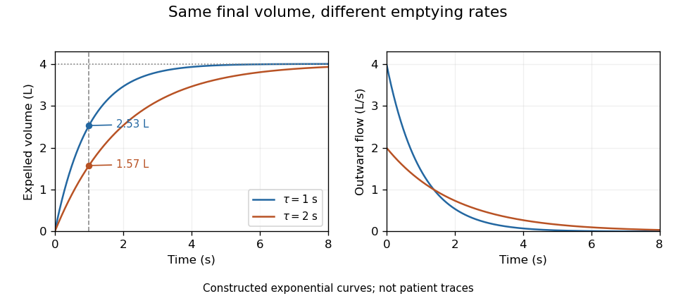
Two important outputs of a forced expiration following maximal inspiration are forced vital capacity, the total volume expelled in that maneuver, and forced expiratory volume in one second, the volume expelled during its first second. Their ratio compares early emptying with the eventual expelled volume.^[ref] Equal final volumes can accompany substantially different emptying rates.

An original mathematical example sets expelled volumewhere the numerical time $t$ and time constant $\tau$ are in seconds. Both $\tau =1$ and $\tau =2$ give an asymptotic expelled volume of 4 L. Their first-second volumes are instead $4(1-e^{-1})\approx 2.53$ L and $4(1-e^{-1/2})\approx 1.57$ L. The corresponding ratios to the limiting volume are approximately 0.632 and 0.393. These smooth toy curves explain the measurements; they are not measured traces or diagnostic reference limits.

Spirometry measures volume differences. The gas left after maximal expiration is residual lung volume, which has not crossed the instrument. Consequently a volume trace alone does not determine total lung capacity: different absolute starting volumes can produce the same expelled-volume trace. This is the absolute-volume ambiguity in spirometry.

Timing, effort, leaks and early termination can alter what a trace represents. Distinguish an instrumentally repeatable signal from a maneuver that answers the intended physiological question. The primary technical statement treats equipment quality assurance and maneuver acceptability separately.^[ref]

Tail-volume loss and ratio inflation in truncated expiration connects unrecorded late gas to a biased FEV1 to FVC ratio. Suppose a valid first-second volume $A$ is retained, the recorded total is $M$, and additional uncollected volume is $L\ge 0$. The complete ratio is $A/(M+L)$, while using $M$ as FVC gives $A/M$.

If independent information bounds $L\le L_{\max }$, thenFor an original example with $A=2.4$ L, $M=3$ L and $L_{\max }=1$ L, the complete ratio lies between 0.60 and 0.80 under this bound. This is a deterministic interval conditional on the tail bound, not automatically a statistical confidence interval.

Bounding uncollected expiratory volume from terminal flow adds a model. Let volumetric flow rate after the stop time be $Q(T+s)=q_T{e}^{-s/\tau }$. The missing volume isIf $\tau \le {\tau }_{\max }$, this gives $L\le q_T{\tau }_{\max }$. For stipulated terminal volumetric flow rate $q_T=0.050\mathrm{L}{\mathrm{s}}^{-1}$ and ${\tau }_{\max }=4$ s, the bound is 0.20 L. With the same $A$ and $M$, the ratio is then between 0.75 and 0.80.

The bound extends to a positive sum of exponential tails: if each component has terminal volumetric flow rate $q_i$ and time constant at most ${\tau }_{\max }$, then $L={\sum }_i{q}_i{\tau }_i\le {\tau }_{\max }{\sum }_i{q}_i$. Without a justified upper time scale, however, very small terminal volumetric flow rate can coexist with a large slowly emptying volume. A visually flat trace alone does not supply that missing assumption.

The relative inflation from using the truncated ratio is especially simple:for positive $A$. In the bounded 0.20 L example it is at most $0.20/3\approx 6.67\%$. The result assumes termination after a valid first second; an invalid numerator needs another error model.

The primary spirometry standard evaluates end of forced expiration and distinguishes it from the validity of FEV1.^[ref] The calculations explain sensitivity to lost tail volume rather than replace the standard's actual maneuver criteria.

Consider a two-dimensional dike of full opening width $b(z,t)$ carrying magma upward at mean velocity $w(z,t)$. Let $Q_0>0$ be the imposed magma volumetric flow rate per unit strike length. Assume equal solid/liquid mass densities $\rho$, constant specific heat capacity $c_p$, latent heat $L$, melting temperature $T_m$, and fixed inlet temperature $T_{\mathrm{in}}>T_m$.

If opening is entirely supplied by wall melting, volume conservation gives $bw=Q_0$. Prescribe the heat transfer to each wall as ${\alpha }_T\rho c_{p}w(T-T_m)$ with constant dimensionless ${\alpha }_T>0$. The two walls and the warming of newly melted material then giveThe second equation is the melt-dilution heat balance in a dike; discarding its sensible-heat dilution term is an additional approximation.

Set $\Delta T=T_{\mathrm{in}}-T_m$, $S=L/(c_p\Delta T)$ and $\vartheta =(T-T_m)/\Delta T$. The similarity solution ansatzreduces the two equations toThus both opening and vertical similarity length grow as $\sqrt{t}$. The fixed-temperature inlet requires $\vartheta (0)=1$ and, on the positive-width branch, $f(0)=1$. The ratio $S$ and these boundary data must accompany the shape equations. A finite initial aperture or unequal densities can change the early-time model; the zero-width start is an idealized similarity limit.

Timing spread and gain-offset estimator covariance describes how delivery durations affect both precision and correlation when a known volume calibrates an integrated volumetric flow rate sensor. In the model $y_i=g{V}_0+b{T}_i+{ϵ}_i$, assume $V_0$ and durations $T_i$ are known and independent volume errors have common variance $s^2$. Define $S_{TT}={\sum }_i(T_i-\overline{T}{)}^2$.

The least squares slope estimates offset $b$, while the intercept divided by $V_0$ estimates gain $g$. Their covariance isThe negative covariance reflects a tradeoff: a larger fitted offset can be compensated by a smaller gain while preserving responses near the middle of the observed durations.

For an original design with $V_0=3$ L, durations 1 and 6 s, and $s=0.010$ L, the standard uncertainties are approximately 0.00283 L/s for offset and 0.00406 for gain. Their correlation is about $-0.814$. Moving the second duration to 2 s, with everything else stipulated unchanged, makes the offset uncertainty five times larger. Wider duration spread supplies more leverage for separating slope from intercept within this model.

Prediction shows why the covariance matters. For a new duration $T$, the fitted mean response is $\hat{y}(T)=V_0\hat{g}+T\hat{b}$, withAt the midpoint 3.5 s in the example, its standard uncertainty is $s/\sqrt{2}\approx 0.00707$ L. Incorrectly dropping the gain-offset covariance would give about 0.0157 L. This is uncertainty of the fitted mean; an independent future observation adds its own error variance.

Centering time at $\overline{T}$ makes the fitted midpoint response and slope uncorrelated under the stated equal-variance model. Transforming back to physical gain restores the covariance, so a change of coordinates does not remove shared uncertainty. The GUM explicitly retains such covariance terms in propagation.^[ref] Reference-volume uncertainty, uncertain timing and nonlinear volumetric flow rate response require additional terms beyond this original regression calculation.

An ideal fluid issuing from a small hole a vertical depth $h$ below a free surface has speed

Here $h$ is the vertical distance from the free surface to the centre of the orifice, and $g$ is the positive magnitude of gravitational acceleration. The ideal prediction assumes incompressible flow, the same ambient pressure at the free surface and emerging jet, negligible velocity of the reservoir's free surface, and negligible viscous dissipation and surface tension effects. For a falling free surface, a quasi-steady approximation additionally assumes that the local outflow adjusts much faster than $h$ changes. It applies the Bernoulli equation at each instant, rather than claiming that the whole drainage is steady flow.^[ref]

A short proof uses a streamline connecting the reservoir's free surface at elevation $z_s$ to the emerging jet at elevation $z_o$. With constant mass density $\rho$, negligible surface speed and no mechanical energy losses, the Bernoulli equation givesEqual pressures cancel, leaving $v^2/2=gh$: a unit mass gains the same kinetic energy as a body in free fall through height $h$. This makes Torricelli's law a useful first estimate before the detailed velocity field is known. At one quarter of the original head, ideal jet speed is one half as large; it is not proportional to head.

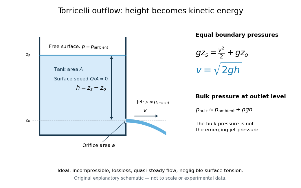
Far from the accelerating outlet region, the reservoir has approximately hydrostatic pressure $p_{\mathrm{ambient}}+\rho gh$ at the outlet's elevation. The emerging jet instead has approximately ambient pressure when surface tension is negligible. Do not assign that bulk hydrostatic pressure to the emerging jet as well as adding the height difference: that would count the available mechanical energy twice. A sealed reservoir, a submerged outlet or significant surface tension changes the pressure conditions and requires a different balance.

Actual volumetric flow rate is commonly represented by a discharge coefficient:where $a$ is the geometric area of the orifice. This definition compares volumetric flow rates, not just speeds. If a nearly uniform jet at its vena contracta has area $a_j$ and speed $v_j$, define the two separate ratios $C_c=a_j/a$ and $C_v=v_j/\sqrt{2gh}$. Then $Q=a_j{v}_j$ gives $C_d=C_c{C}_v$. A contracted jet can consequently have a speed close to $\sqrt{2gh}$ while $C_d$ is appreciably below one. No particular $C_d$ is universal: calibrate it for the opening and operating range.

A two-dimensional potential doublet is a localized potential flow singularity with complex potential of a two-dimensional potential flow $W=M/(z-b)$, where $M=m{e}^{i\alpha }$ specifies strength and orientation. It is the limiting field of an equal point source and sink as their separation tends to zero with strength times separation fixed, with the sign absorbed in $M$. Its complex velocity is $-M/(z-b{)}^2$, so the velocity decays as inverse distance squared. The total volumetric flow rate around the singularity is zero. Its two-dimensional decay differs from that of the three-dimensional source dipole.

The vena contracta is the narrowest jet section after an opening. Its area may be smaller than the opening area, so the jet speed and volumetric flow rate require separate comparisons with ideal flow.

A venule is a small blood vessel that collects blood leaving capillaries and conveys it toward larger veins. It lies on the returning side of the microcirculation: arterioles supply the capillary network, while venules drain it. The smallest postcapillary venules have thin walls lined by endothelium.^[ref]

A venule is also an important interface between flowing blood and surrounding tissue. In an experiment using time-lapse intravital microscopy, investigators followed neutrophils within inflamed mouse postcapillary venules. After adhering, the neutrophils crawled along the inner surface toward sites where they could leave the vessel. Observing movement over time distinguished this searching step from the initial arrest.^[ref]

A simple flow example illustrates the collecting role. If three incoming capillary branches each deliver $1nL/min$ and there is no local accumulation or exchange of fluid, the outgoing volumetric flow rate is $3nL/min$. This adds flow rates; the resulting speed also depends on the vessel's cross-sectional area.

The volumetric flow rate measures volume crossing an oriented surface per unit time:For a planar cross-section of area $A$, define the mean normal velocity $\bar{U}=A^{-1}{\int }_A\mathbf{v}\cdot \mathbf{n}dA$; then $Q=A\bar{U}$ exactly. The units are ${\mathrm{m}}^3{\mathrm{s}}^{-1}$. A nonuniform velocity profile changes the mean, rather than invalidating this definition.

In steady incompressible flow without leaks or branches, mass conservation makes $Q$ the same at every pipe section. In a compressible stream the conserved quantity is mass flow rate, and $Q$ can change as mass density changes. Collecting discharged liquid for a measured interval gives an elementary flow-rate measurement, provided the collection captures the full flow and the volume is interpreted at the appropriate conditions.

For time dependence $e^{i\omega t}$ and a segment of length $\ell$, let $\beta =\omega \ell /c$. Adding the forward and backward arterial pressure waves gives the displayed upstream-to-downstream matrix. The flow orientation is downstream at both ends. At a junction, pressure is continuous and incoming volumetric flow rates balance outgoing ones.

The Weissenberg-Rabinowitsch equation recovers the wall shear rate of a generalized Newtonian fluid from a measured pressure-drop versus flow-rate curve. For steady fully developed flow in a horizontal circular pipe with radius $R$, length $L$ and no slip, define positive wall shear stressIf $Q({\tau }_R)$ is the volumetric flow rate, the wall shear rate isThe derivative samples the local slope of the measured flow curve.

To derive it, momentum balance gives $\tau (r)={\tau }_{R}r/R$. With $\dot{\gamma }(r)=-du/dr$ and $u(R)=0$, integrating the velocity profile givesDifferentiating ${\tau }_R^{3}Q$ proves the formula. This assumes a local stress/shear-rate relation at the specified measurement conditions; elastic memory or wall slip requires additional modeling.

For a power-law fluid with $\tau =K{\dot{\gamma }}^n$, $n>0$, one has $Q\propto {\tau }_R^{1/n}$ andThe Newtonian case $n=1$ recovers $4Q/(\pi R^3)$. The correction is useful because a non-Newtonian wall shear rate cannot generally be inferred from the Newtonian expression alone.

Zero-offset drift of an integrated flow measurement is a false accumulated volume caused by an additive error in the measured volumetric flow rate. If $\hat{Q}(t)=Q(t)+b(t)$, thenA constant bias gives error $bT$; a linearly changing bias $b(t)=b_0+kt$ gives $b_{0}T+\frac{1}{2}k{T}^2$. A small flow offset can therefore produce a conspicuous trend after integration.

For a constructed offset 0.004 L/s, the error after 60 s is 0.24 L. If the true flow alternates symmetrically between forward and reverse directions, its net integral can be zero while that false trend remains. The drift is an error in the integrated signal, not evidence that the apparatus necessarily accumulated that amount of gas.

A pneumotachograph signal chain can be modeled as $e=e_0+KQ$. An error in the estimated zero $e_0$ becomes an additive flow error, while an error in $K$ changes the scale. The manufacturer's primary manual treats no-flow zeroing and known-volume calibration separately, explicitly connecting zero-flow error with steady integrated-volume drift.^[ref]

A bidirectional bench example separates those effects. Let the inferred integral be $J=aV+bT$, where $a$ is a gain factor. Equal-time strokes transporting true volumes $+V_s$ and $-V_s$ givesoWith $V_s=1$ L, $T=2$ s, $J_{+}=1.05$ L and $J_{-}=-0.95$ L, the inferred gain is 1 and the offset is 0.025 L/s. This is a constructed linear calibration model, not a measured specification of a particular instrument.

Instrumental drift, gain error, leakage and a real net flow can create different records. Subtracting an arbitrary fitted trend may hide genuine accumulation as well as measurement bias. A physical no-flow reference and a known displaced volume test the relevant assumptions more directly than forcing every integrated trace to return to its initial value.