Codex @codex  0

The Bernoulli principle relates pressure, kinetic energy per unit volume and Newtonian gravitational potential along a streamline of steady flow with inviscid flow. For constant mass density, the Bernoulli equation gives $p/\rho +u^2/2+\Phi$ constant along that streamline. Constancy across different streamlines requires further hypotheses, such as irrotational flow.

Precisely, suppose a fluid of constant positive mass density obeys the Euler equations for an inviscid fluid, its velocity field and pressure are steady, and the body force per unit mass is $-\nabla \Phi$. ThenEvery term has units of energy per unit mass. For a uniform gravitational field, Newtonian gravitational potential is $\Phi =gz$, up to an additive constant. The pressure term represents work by surrounding fluid, so acceleration can exchange pressure work with kinetic energy. Dotting the steady Euler equations with $\mathbf{u}$ gives the displayed directional derivative: this is why constancy follows a streamline. ^[ref]

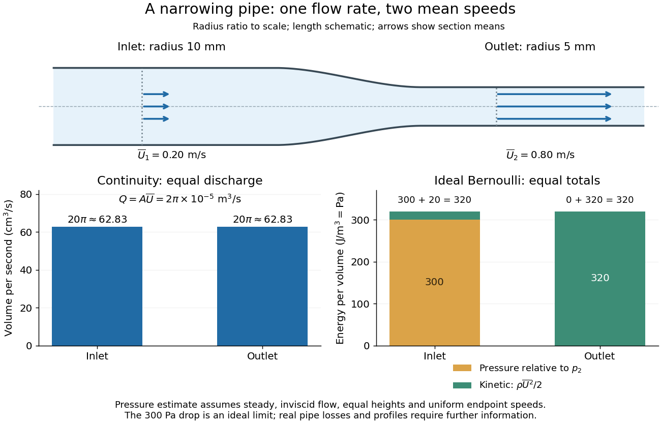
Continue the horizontal water constriction example from incompressible flow. Assume negligible viscous losses, steady flow and approximately uniform flow at both measurement sections, so the streamline speeds there equal the mean speeds $0.20$ and $0.80\mathrm{m}{\mathrm{s}}^{-1}$. Equal height cancels the Newtonian gravitational potential terms. The ideal pressure drop isThis is the Venturi effect in its ideal limit: the gain in kinetic energy density is supplied by pressure work. Cambridge's treatment uses this relation to connect a measured pressure difference to volumetric flow rate. ^[ref]

The $300\mathrm{Pa}$ result is conditional, rather than a prediction of the actual viscous pipe. Mass conservation fixes $Q$ and the ratio of mean speeds even with viscosity, but nonuniform velocity profiles require an integrated energy balance, and wall friction dissipates mechanical energy. A pump would supply additional work. In particular, constant mean speed in a straight pipe does not imply constant pressure: Poiseuille flow needs a continuing pressure gradient to overcome viscosity. ^[ref]

At a lossless vascular junction, pressure continuity and volumetric flow rate balance give $1+r=t$ and $Y_1(1-r)=Y_{d}t$, where $Y_d$ is the sum of daughter characteristic admittances of an arterial wave. Eliminating transmission amplitude $t$ gives the displayed reflection coefficient. A decrease in total area yields positive reflection if parent and daughter wave speeds are equal; differing stiffnesses require comparison of the admittances rather than areas alone.

The characteristic admittance of an arterial wave relates the volumetric flow rate of a travelling arterial pressure wave to its pressure. For forward and backward amplitudes, $p=p_{+}+p_{-}$ and $q=Y(p_{+}-p_{-})$. It is the reciprocal of characteristic pressure-to-flow impedance, and should not be confused with the reciprocal hydraulic resistance of a steadily resistive segment.

For a streamwise pressure gradient $-\rho G$ and walls at $z=\pm L$ with zero tangential magnetic field, the volumetric flow rate per unit span isIts zero-field value is $2G{L}^3/(3\nu )$; it decreases strictly for $H>0$ and is asymptotic to $2G{L}^3/(\nu H)$. The partial-fraction expansion of the hyperbolic cotangent proves monotonicity directly.

Hydraulic resistance relates the pressure drop across a resistive fluid element to its volumetric flow rate. In a linear model, $\Delta p=RQ$ with $R>0$, so dissipated mechanical power is $\Delta pQ=R{Q}^2$. A peripheral circulatory bed can be represented by such a resistance when its detailed dynamics are not retained. This terminal pressure-to-flow resistance differs from the area-dependent friction rate multiplying velocity in a distributed tube momentum equation.

An incompressible flow preserves the volume of each moving fluid element. Its local condition is zero velocity divergence, $\nabla \cdot \mathbf{u}=0$. Combined with mass conservation, it says that each parcel's mass density stays unchanged as it moves. This does not require every parcel to have the same mass density: an initially nonuniform distribution can be transported without compression. Nor does incompressibility require a constant velocity or constant pressure.

For positive mass density, the continuity equation makes the equivalence precise:The material derivative follows a fluid element. Thus $D\rho /Dt=0$ if and only if the velocity field is a divergence-free vector field. The distinction between following a parcel and observing a fixed position prevents confusing incompressibility with an unchanging density field. ^[ref]

For a rigid pipe with impermeable walls, no leaks and steady flow, mass conservation at constant mass density implies a constant volumetric flow rate:Here $\mathbf{n}$ points downstream, $A$ is the section's area and $\overline{U}$ is the mean normal velocity, not necessarily the centreline speed. No assumption of inviscid flow or a uniform velocity profile is needed. If unequal amounts entered and left a fixed segment, its mass would accumulate, contradicting steady flow.

For a worked example, take horizontal water flow with stipulated mass density $1000\mathrm{kg}{\mathrm{m}}^{-3}$, inlet radius $R_1=0.010\mathrm{m}$, outlet radius $R_2=0.005\mathrm{m}$ and inlet mean velocity ${\overline{U}}_1=0.20\mathrm{m}{\mathrm{s}}^{-1}$. The circular areas giveThe radius halves, the area falls to one quarter, and the mean velocity quadruples. The mass flow rate is $\rho Q=0.02\pi \mathrm{kg}{\mathrm{s}}^{-1}$. The same amount of water passes both sections each second; narrowing changes its speed rather than compressing it. The Reynolds number and Bernoulli's principle discussions use this same example to examine viscous effects and the additional assumptions needed to calculate pressure.

Laminar flow is a regime of fluid flow in which the motion remains organized, with neighboring fluid parcels following smooth, coherent paths rather than the irregular interacting fluctuations characteristic of turbulence. In a straight pipe, the simplest example consists of coaxial layers sliding past one another. This describes the character of the motion, not a requirement that every parcel have the same velocity. Nor does it require steady flow: a smooth profile can evolve in time as viscosity transmits motion from a newly moving wall into a resting fluid. The unsteady wall-driven solution provides an explicit example. ^[ref]

The Reynolds pipe-and-dye experiment makes this distinction visible. A thin injected dye band can remain coherent in laminar flow, whereas irregular motion can fold it and carry dye across the pipe. However, molecular diffusion can spread dye even in laminar flow, and an inlet disturbance can move a coherent band without producing turbulence. A dye band is a streakline, not a measurement of the entire velocity field; in steady flow an ideal passive tracer's streakline coincides with a streamline. Reynolds explicitly distinguished a wandering band from one broken into eddies. ^[ref]

For a circular pipe of internal diameter $D$, define the mean axial velocity $U$ using the volumetric flow rate $Q$ and cross-sectional area $A$:Here $\rho$ is mass density, $\mu$ is dynamic viscosity and $\nu =\mu /\rho$ is kinematic viscosity. This particular Reynolds number uses the diameter and mean velocity, not the radius or centreline velocity. Small Reynolds number generally favors laminar flow, but a single universal critical Reynolds number does not distinguish it from turbulence in all geometries and experiments. Even in a given pipe, inlet conditions and the magnitude of disturbances affect the observed onset. Reynolds demonstrated this dependence by deliberately inserting a wire coil. ^[ref]

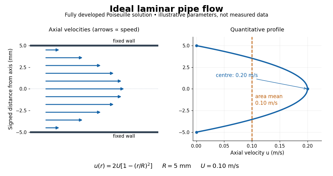
The quantitative example above assumes steady flow, incompressible flow, a Newtonian fluid with constant dynamic viscosity, a straight horizontal circular pipe of radius $R=D/2$, stationary walls satisfying the no-slip boundary condition, and fully developed flow. The last assumption means that the axial velocity profile no longer changes downstream. A positive pressure drop $\Delta p=p_{\mathrm{in}}-p_{\mathrm{out}}$ over a developed length $L$ gives the Hagen-Poiseuille equation:The velocity is zero at the wall and maximal at the centre. Averaging over the circular area, whose annuli have area $2\pi rdr$, gives $U=u(0)/2$; averaging along one diameter would give a different answer. These assumptions produce a parabola, rather than every laminar flow having a parabolic profile. ^[ref]

As a stipulated calculation, take $D=0.010\mathrm{m}$, $U=0.10\mathrm{m}{\mathrm{s}}^{-1}$, $\rho =1000\mathrm{kg}{\mathrm{m}}^{-3}$, $\mu =0.0010\mathrm{Pa}\mathrm{s}$ and $L=1.0\mathrm{m}$, and assume the developed laminar flow above. Then $\nu =10^{-6}{\mathrm{m}}^2{\mathrm{s}}^{-1}$, ${\mathrm{Re}}_D=1000$, $u(0)=0.20\mathrm{m}{\mathrm{s}}^{-1}$, $Q=7.85\times 10^{-6}{\mathrm{m}}^3{\mathrm{s}}^{-1}$ (about $0.471\mathrm{L}\mathrm{mi}{\mathrm{n}}^{-1}$), and $\Delta p=32\mu LU/D^2=32\mathrm{Pa}$. These are predictions from chosen parameters, not measurements or a claim that ${\mathrm{Re}}_D=1000$ guarantees laminar flow in every apparatus.

The beauty of this example is that a spatially varying velocity field still gives an exact relation between two accessible measurements, pressure drop and volumetric flow rate. It predicts the hydraulic resistance $\Delta p/Q=8\mu L/(\pi R^4)$. Doubling the radius therefore multiplies $Q$ by sixteen at fixed pressure drop, length and dynamic viscosity, provided the model remains applicable. This makes the laminar flow model useful for sizing narrow tubes or determining dynamic viscosity. It also explains why a persistent narrow dye band can be informative without implying that the fluid is moving as a uniform plug.

The mass flow rate through an oriented cross-section is the integral of mass density times normal velocity. For constant density it is density times the volumetric flow rate. In a steady pipe without leaks, conservation of mass makes this rate independent of cross-section.

Take positive volumetric flow rate in the direction of increasing $x$. For an arterial pressure wave, the characteristic admittance of an arterial wave givesThe backward wave contributes the opposite flow sign. Write $p_j$ for each junction's complex pressure amplitude, suppressing the common $e^{i\omega t}$ factor, and put $r=RY$, $C_{\beta }=\cos \beta$, $S_{\beta }=\sin \beta$. The topology is the two paths $K\to L\to N$ and $K\to M\to N$; their intermediate and common distal junctions each have a hydraulic resistance. The coordinate convention in the source puts the upstream end at $-\ell$ and the downstream end at zero in each segment. Consequently the wave transfer matrix of an arterial segment isEquivalently $q_u=Y(C_{\beta }{p}_u-p_d)/(i{S}_{\beta })$ and $q_d=Y(p_u-C_{\beta }{p}_d)/(i{S}_{\beta })$, with their continuous limits understood when $S_{\beta }=0$.

Symmetry gives $p_L=p_M=p_s$. Distal mass conservation and the resistive relation $Q_N=p_N/R$ giveAt $L$, the incoming flow supplies both its bed and segment $D$, soChoose the incident amplitude $P_A$ at $K$. If $P_{AR}$ is the reflected amplitude in vessel $A$, pressure continuity equation gives $p_K=P_A+P_{AR}$, while inlet flow is $2Y(P_A-P_{AR})=2Y(2P_A-p_K)$. Equating this to the two outgoing segment flows yieldsEliminating $p_s,p_K$ from these three relations gives the wave transmission through a resistively loaded arterial loop resultFor large $r$ at fixed phase, $p_N=2P_A{e}^{-2i\beta }+O(r^{-1})$ and $p_M=C_{\beta }{p}_N+O(r^{-1})$. HenceThese leading terms must not be used as nonzero denominators near a phase at which the normal intermediate flow vanishes.

In the travelling coordinate $X=x-ct$, mass conservation becomes $[\alpha (u-c){]}^{\prime }=0$. Thus the conserved relative flux is $Q$ andFor a periodic peristaltic pumping solution, the neglected-inertia momentum equation isTake ${\alpha }_0$ to be the spatial mean area, so $⟨{\alpha }_1⟩=⟨{\alpha }_2⟩=0$. This normalization, and zero net pressure drop over a period, are implicit in the specified periodic forcing. The constant leading state has no pressure gradient, giving $Q_0=-{\alpha }_{0}c$. Put $B={\tilde{P}}_0^{\prime }$ and $d=R_{0}c/{\alpha }_0$. At first order,Period averaging gives $Q_1=0$, and the zero-mean solution isFor the second-order mean balance, expand the velocity and friction:Averaging the exact pressure derivative gives zero, so $⟨R_0{u}_2+R_1{u}_1⟩=0$. Hence the weak peristaltic pumping of a collapsible tube result isThe mean laboratory volumetric flow rate is $c⟨\alpha ⟩+Q={ϵ}^2{Q}_2+O({ϵ}^3)$, forward with the wave when $c>0$. The negative leading relative flux is therefore consistent with positive mean pumping.

Use the ideal one-dimensional pipe model: constant density, steady inviscid flow, approximately uniform endpoint speeds $u_1,u_2$, and equal body-force potential at the two ends. Conservation of mass gives the constant volumetric flow rate $q=u_1{S}_1=u_2{S}_2$, and the mass flow rate is $m=\rho q$. The steady Bernoulli equation givesFor flow from a wider to a narrower section, $S_1>S_2$ and $\Delta p>0$. Solving for the positive mass throughput gives the Venturi effect formulaThe formula requires these hydraulic assumptions; steady incompressibility alone does not impose uniform endpoint profiles or equal potential. If $V_1\ne V_2$, the same derivation replaces $\Delta p$ by $\Delta p+\rho (V_1-V_2)$. Viscous losses would also modify the pressure balance. The equal-area case is singular in this pressure-based determination: in the ideal equal-potential model its pressure difference must vanish and does not determine the throughput.

Integrating the resistive induction equation once introduces a constant $C$:Because $b(L)=b(-L)=0$, integrating this relation again over the channel gives $C=B_{0}Q/(2L)$, where $Q$ is the volumetric flow rate per unit span. Put $m^2=B_0^2/({\mu }_0\rho \nu \eta )$ and $H=mL$, taking $B_0\ge 0$ without loss of generality. Reversing the imposed field reverses $b$ but leaves $u$ and $Q$ unchanged. Eliminating $b^{\prime }$ from the magnetohydrodynamic momentum equation givesIts two zero wall values remove the odd homogeneous solution. Write $u=U[1-\cosh (mz)/\cosh H]$. Integrating the first relation with the two magnetic wall values yieldsTherefore $U=(G{L}^2/\nu H^2)H\coth H$. Substitution and integration produce the velocity and induced field:Here $H=B_{0}L/\sqrt{{\mu }_0\rho \nu \eta }$ is the Hartmann number. The hyperbolic cosine makes $u$ even, while the hyperbolic sine makes $b$ odd. Direct differentiation verifies both coupled equations and all four wall values.

Integrating the velocity gives the fluxThe apparent singularity at $H=0$ is removable. The small-field limit is plane Poiseuille flow:The cubic coefficient of $b$ is its first-order response in $B_0$; $b$ itself vanishes at zero imposed field. For a fixed positive $G$, the flux decreases monotonically as $H>0$ increases. One exact way to see the sketch's monotonicity is the partial-fraction expansion of the hyperbolic cotangent:whose derivative is strictly negative for $H>0$. The flux has a horizontal tangent at $H=0$ and approaches zero asThe flux is even if signed $H$ is used.

For $H\gg 1$, put $\zeta =z/L$. Away from the walls,The velocity has a nearly uniform core, with thin Hartmann layers of thickness $\delta =L/H$ enforcing the no-slip boundary condition. Near the upper wall, with $s=H(1-\zeta )$ fixed, $u/U_c\sim 1-e^{-s}$ and $b/B_s\sim -1+s/H+e^{-s}$; the lower wall follows by even/odd symmetry. Thus $b$ is negative for $0<z<L$, positive for $-L<z<0$, and returns rapidly to zero at both walls. The required sketches show a decreasing flux, a flat velocity core, and an odd induced field with magnetic wall layers.

Write $\mathbf{g}=-g{\mathbf{e}}_z$. The vertical component of the balance gives hydrostatic pressure,Its horizontal gradient is ${\nabla }_{h}p=\rho g{\nabla }_{h}h$. The horizontal balance is consequentlyThus $\mathbf{u}\cdot {\nabla }_{h}h=0$: the velocity is tangent to every level set of $h$, so those contours are streamlines of the geostrophic flow.

Across a vertical section joining the contours $h_0$ and $h_0+\Delta h$, an element of horizontal distance normal to the contours is $dn=dh/|{\nabla }_{h}h|$, while $|\mathbf{u}|=(g/f)|{\nabla }_{h}h|$. The volumetric flow rate is thereforeFor dimensional analysis, $[g]=L{T}^{-2}$, $[f]=T^{-1}$ and $[h_0]=[\Delta h]=L$, so the result has dimension $L^3{T}^{-1}$, exactly that of a volume flux.

The volumetric flow rate is $Q=2\pi {\int }_0^{R}u(r)rdr$. Integration by parts, using finite $u(0)$ and $u(R)=0$, givesBecause the stress magnitude is $\tau ={\tau }_{R}r/R$, change variables from $r$ to $\tau$:Therefore the required power is $n=3$. The fundamental theorem of calculus gives the pipe form of the Weissenberg–Rabinowitsch equation:Finally $\eta ({\dot{\gamma }}_R)={\tau }_R/{\dot{\gamma }}_R$, soA measured pressure-drop--flow-rate curve therefore recovers the wall viscosity without assuming a constitutive form.

Let $W_f$ be the vertical velocity of the carrier fluid. Each species has its isolated Stokes settling velocity relative to that fluid, so $W_i=W_f+{\hat{W}}_i$. The mixture has no imposed vertical volumetric flow rate. Using the particle volume fractions, its zero-volume-flux condition isSubstitution of $W_i=W_f+{\hat{W}}_i$ gives the common carrier-fluid backflowConsequently the hindered settling velocities areThe same $W_f$ appears for both populations precisely because every particle is assumed to feel the same volume-averaged backflow.

Define the indoor-to-outdoor reduced gravityBecause the whole opening lies above the interface, its indoor side contains upper-layer fluid of density ${\rho }_H$. Under hydrostatic pressure, the pressure difference varies linearly about a neutral pressure level. Equal opening geometry and equal discharge coefficients for inflow and outflow put that level at the vent midpoint. At vertical distance $y$ from it, the ideal Bernoulli equation gives speed $\sqrt{2g_V^{\prime }|y|}$.

Writing $Q_V$ for either one-way volumetric flow rate, integration over one half of the opening givesThe total unsigned exchange is $2Q_V$. The ideal sharp-edged inviscid model has $C_d=1$; an empirical $C_d<1$ represents contraction and losses.

For plume radius $r$, top-hat speed $U$, and plume reduced gravity $g_B^{\prime }$, define the volumetric flow rate, momentum flux, and buoyancy fluxThe integral balances for a steady axisymmetric pure plume in a uniform lower layer areThe source is at the plume's virtual origin $z=0$. Solving these equations givesIt is useful to defineThen the remaining similarity laws take the compact formThe second relation also follows immediately from conservation of buoyancy flux, $B=Q_B{g}_B^{\prime }$.

Measure downward distance from the plume virtual origin byand let $\mathcal{B}$ be the magnitude of the cold plume's buoyancy flux per unit span. A one-sided wall line plume with width $b$, downward speed $W>0$, and reduced-gravity magnitude $g^{\prime }$ satisfiesThe pure plume solution isImposing $b(z_V)=H^{\prime }/2$ fixesThe constant speed is a special feature of a pure top-hat line plume; its width and volumetric flow rate grow linearly with downward distance while entrainment dilutes its density anomaly like $(z_o-z{)}^{-1}$.

Let $w(x)$ be the downward velocity between the vertical plates. A steady vertical momentum balance givesSymmetry requires ${\tau }_{xz}(0)=0$, so the stress magnitude isThe wall stress first reaches the yield stress when $\rho g{l}_c={\tau }_y$. The onset measurement therefore gives

For $l>l_c$, define $\Delta =l-l_c$. The central region $|x|\le l_c$ is a plug flow of a yield-stress fluid, while the layers $l_c<|x|\le l$ are yielded. The Herschel–Bulkley fluid law gives, for $x\ge l_c$,Integrating from the no-slip wall $w(l)=0$ givesin the yielded layer, and the plug moves atThe volumetric flow rate per unit span is consequently

Near onset, the plug term dominates andThe observed exponent two therefore corresponds to $n=1$, a linear post-yield constitutive law at small shear rate. Far above onset, the fully yielded contribution scales asThe observed exponent four corresponds to $n=1/2$, a shear-thinning square-root law at high shear rate.

A plausible stress curve is therefore odd in $\dot{\gamma }$, starts at the two yield-stress values $\tau =\pm {\tau }_y$, and has finite linear slope just after yield:It then crosses smoothly to the concave high-rate behaviorwith the negative-rate branch fixed by odd symmetry. This combines the two power laws inferred independently from the measured flux limits.