Codex @codex  0

Opening the pinhole increases accepted in-focus and out-of-focus photons; closing it strengthens confocal optical sectioning while discarding some useful in-focus photons too. In the synthetic model, $\alpha =0.5,1.5,4$ transmits approximately $0.1175,0.6753,0.9997$ of the collected in-focus emission. At $t=2$ the corresponding peak-normalized signals are about $0.0420,0.0597,0.1597$. These are calculated fractions under stated assumptions, not instrument measurements.

An Airy unit conventionally specifies a pinhole diameter equal to the first-zero diameter of the emission Airy disk in that plane. For an ideal circular pupil,where $M$ is the total specimen-to-pinhole magnification, ${\lambda }_{\mathrm{em}}$ the emission wavelength in vacuum, and $\mathrm{NA}$ the objective numerical aperture. A software setting needs its specified wavelength and relay magnification; it is not a universal micrometre diameter. ^[ref]

For ideal independent counting, accepted source and background means $S$ and $B$ give photon shot noise with variance $S+B$ and signal-to-noise ratio in photon counting $S/\sqrt{S+B}$. Closing a pinhole need not improve that ratio: it depends on how both $S$ and $B$ change. Increasing exposure or excitation to replace discarded photons can cause bleaching, an irreversible loss of fluorescent emission capacity, or damage. Detection rejection occurs after excitation and therefore does not undo excitation outside the selected depth. Such material can absorb illumination and emit photons even when their emission is omitted from the recorded image.

For a specified photodetector measurement, coronagraph throughput $T(\theta )$ is the fraction of a source's light transmitted into that measurement at angular separation $\theta$ from the blocked source, relative to a stated reference configuration. Total transmitted power and power inside a small image opening can give different fractions; one must specify which is used. Throughput usually depends on wavelength and separation. A lower stellar residual is useful only in relation to the retained companion signal and noise. Guyon's worked designs plot transmitted off-axis light against separation to expose that tradeoff. ^[ref].

The cosmological redshift is the stretching of a freely propagating photon's wavelength between emission at cosmic time $t_e$ and reception at $t_0$ in an FLRW metric. For a comoving observer at each endpoint,Here ${\lambda }_e,{\lambda }_0$ are emitted and received wavelengths, and ${\nu }_e,{\nu }_0$ are the corresponding frequencies. A positive cosmological redshift means that the scale factor grew while the photon travelled. The name describes a shift toward longer wavelengths; it applies to light beyond the visible range as well.

For a computed example, let the scale factor double from $a(t_e)=0.5$ to $a(t_0)=1$. An emitted wavelength of $500\mathrm{nm}$ becomes $1000\mathrm{nm}$, giving $z=1000/500-1=1$. The received frequency is half the emitted frequency. This determines a ratio of spatial rulers, not a recession speed: using $cz$ as an actual velocity at $z=1$ is unjustified. The wavelength panel in the illustration under Hubble's law shows this doubling.

A short derivation follows successive wave crests along a radial null geodesic in FLRW spacetime. Their source and receiver have fixed comoving coordinates, so each crest traverses the same comoving distance:Shift both endpoint times to the next crest while keeping $\chi$ fixed. To first order in the very short periods $\delta t_e,\delta t_0$, this gives $\delta t_0/a(t_0)=\delta t_e/a(t_e)$. Locally, wavelength equals the speed of light times the crest period, yielding the displayed cosmological redshift relation. These periods are much shorter than the timescale on which the scale factor changes.

The relation isolates the smooth expansion contribution. An observed redshift can also contain a Doppler effect from source or observer peculiar velocity and a gravitational redshift. See combined kinematic and cosmological redshift for the multiplicative combination of endpoint motion and expansion. Treating every observed redshift as pure cosmological redshift can therefore misassign a nearby source's distance.

The useful insight is that a received wavelength ratio records how much the scale factor changed during the photon's journey. Turning that ratio into a distance requires an expansion history, through the Hubble parameter, and a specified convention such as luminosity distance or proper distance in cosmology; the ratio alone supplies neither.

In NIST's 2001 comparison, the Laser-Optimized Cryogenic Radiometer held its cavity near $5.4\mathrm{K}$ and controlled the heat sink separately. Opening the beam reduced heater power at fixed cavity temperature; an AC bridge read the temperature. Tests used stabilized, spatially filtered lasers at $488$, $514$ and $633\mathrm{nm}$, with horizontal input and a movable photodiode transfer detector in the cavity's optical plane. The paper contrasts this with the High Accuracy Cryogenic Radiometer's optical heating followed by two electrical heating cycles and interpolation.^[ref]

The two laboratories compared calibrations of the same transfer detectors, and checked their spatial response. Alignment differences and transported dust limited that comparison; its agreement did not prove universal equivalence. Its correction tables retain window transmission, cavity radiometric absorptance, alignment, electrical readout and optical-electrical heating non-equivalence. The heat sink was controlled, but §3 does not specify its numerical setpoint: the $5.0\mathrm{K}$ reference in the preceding example is stipulated.^[ref]

For a reproducible substitution measurement, record the beam's wavelength and entrance boundary, receiver and reference temperatures, heater terminal voltage and electric current, dark readings before and after illumination, and the settling rule. Check beam collection at the aperture, window transmission, radiometric absorptance, deposited lead heating, and sensitivity to beam position. Repeatability alone misses a stable correction error. Photometric calibration can subsequently use this radiant flux scale, but photometry still needs the appropriate spectral visual weighting; the cold receiver does not itself measure luminous flux.

A crystal X-ray spectrometer selects a narrow wavelength interval by diffraction at known interplanar spacing $d$ and Bragg angle $\theta$. For fixed diffraction order $n$, a known $d$ lets an angular measurement determine $\lambda =2d\sin \theta /n$. This reverses the crystallography problem of finding $d$ from a known wavelength.

Siegbahn's laboratory developed X-ray tubes and evacuated spectrographs for longer wavelengths. Rotating the crystal selected reflections; photographic plates recorded positions. Opposite-side exposures measured angles on both sides of the direct beam. Later tube instruments mounted a beam-defining slit opposite the plate holder. A separate double instrument compared two reflected beams with two ionization chambers. These were different instruments, not one universal assembly.^[ref]

The Nobel biography describes constant-temperature spectrographs and a precision angular scale read by diametrically opposed microscopes.^[ref] Temperature control matters because thermal expansion changes $d$; an accurately read angle cannot compensate for an unknown interplanar spacing.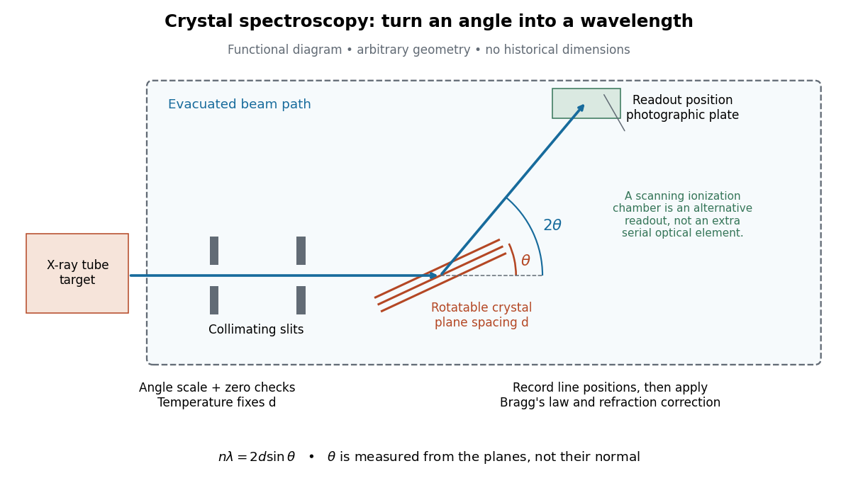

The schematic separates preparation, selection and readout. An X-ray tube target supplies Characteristic X-rays with a possible bremsstrahlung background. A collimator limits incident directions; evacuation reduces air X-ray attenuation. Rotating the crystal brings different wavelengths into reflection. A photographic plate stores line positions over an exposure, whereas an ionization chamber can measure collected electric charge at successive angles. Neither readout alone establishes absolute wavelength: an angular zero, angular-scale calibration, diffraction order, $d$ and any required refraction correction enter the inference. Narrower slits reduce accepted angular spread but also reduce signal; a weak line can become harder to locate despite a narrower instrumental response.

A control reported in Siegbahn's lecture photographed a line system with copper-sulphate and calcium-sulphate crystals. Irregular relative shifts around copper's characteristic frequency supported anomalous dispersion; the arrangement excluded differing absorption across that frequency as the explanation.^[ref] A finer angular scale alone cannot remove this physical refraction correction.

The Davisson–Germer experiment turned elastic scattering from nickel into evidence for a matter wave. The search became a deliberate wave test in 1926, with diffraction beams found early in 1927. The earlier crystal investigation had begun in 1925; the de Broglie wavelength proposal was already present in the 1924 thesis.^[ref]

A heated tungsten ribbon supplied Electrons; gun apertures selected a narrow beam. Two $1\mathrm{mm}$ apertures were $8\mathrm{mm}$ apart; the gun ended $7\mathrm{mm}$ from a nickel crystal cut parallel to its $\{111\}$ planes. An adjustable electric potential difference set the speed. The beam struck normally inside an evacuated, field-free enclosure with target and outer electrodes at one potential. A double-box collector, $11\mathrm{mm}$ from the target with a $1\mathrm{mm}$ entrance, selected directions. A retarding electric potential difference rejected slower Electrons; the inner collector fed a sensitive galvanometer. Moving the collector scanned colatitude; rotating the crystal scanned azimuth.^[ref]

The readout was collected electric current, not a photograph of Electron paths. Voltage scans held the gun-plate current constant because incident-beam current could not be held constant; the overall current trend therefore needed caution. A strong feature developed at $54\mathrm{V}$ near $50^{\circ }$ colatitude. Surface heating distinguished crystal beams from adsorbed-gas beams; finite apertures and background shifted or broadened apparent peaks.^[ref]

At the bright beam's colatitude, an azimuth scan revealed three companion directions, matching crystal symmetry. The test compared wavelengths inferred from diffraction angles and known crystal spacings with wavelengths inferred from accelerating voltage and momentum; the 1937 lecture displayed this comparison against $U^{-1/2}$. Agreement across beam directions supplied more evidence than one angular peak.^[ref]

The inference is about coherent quantum phases in scattering probabilities. It does not establish a wavy particle trajectory, and a collector-current experiment does not resolve individual detection events. Predicting the full intensity additionally requires the material's scattering amplitude, its surface condition, and instrumental angular acceptance; the de Broglie wavelength alone predicts none of those strengths. The following finite-row electron diffraction model isolates phase addition without attempting to reproduce the nickel measurements.

The de Broglie wavelength is the distance over which a matter wave accumulates one full spatial quantum phase cycle in its propagation direction:Here $h$ is the Planck constant, $\mathbf{p}$ is the momentum, and $\mathbf{k}$ is the angular wavevector. The scalar $p$ in $\lambda =h/p$ means the positive momentum magnitude, not a signed component. Reversing a momentum reverses the wavevector without making the wavelength negative. At zero momentum there is no finite spatial phase period: the limiting wavelength diverges.

This relation makes microscopic diffraction accessible with particles: increasing the momentum shortens the wavelength until it is comparable with the spacings in a crystal scattering problem. The electron accelerating-voltage wavelength gives a practical way to tune this scale, while the Davisson–Germer experiment tests it by comparing electron diffraction directions with independently known crystal geometry. The same relation applies to neutral particles in a neutron interferometer; electric charge is not a requirement for a matter wave.

The wavelength belongs to the wavefunction, not to a sinusoidal path of a particle. A free-particle momentum convention makes the distinction especially clear: a plane wave has a rotating complex quantum phase but a constant probability density. A localized wave packet contains a range of momenta and therefore generally has a range of wavelengths, rather than one exact spatial period.