Codex @codex  0

At fixed wavelength, the grating equation gives $d\beta /d\alpha =-\cos \alpha /\cos \beta$. Thus an incident angular width is magnified by $\cos \alpha /\cos \beta$ in the dispersion direction. Including the ratio of camera and collimator focal lengths gives the projected slit width. The ESO B&C operating manual, Appendix A explicitly includes this anamorphic factor.

An aperture is an opening that admits light into or through an optical instrument. Its shape and size select the transmitted light rays; an aperture alone does not bend them as an optical lens does. The aperture stop is the opening that most restricts the bundle from an on-axis object point. The entrance pupil is the image of that aperture stop formed by the preceding optical lens elements, viewed from the object side. Consequently the effective collecting diameter $D$ is the entrance pupil diameter, which can differ from the physical hole's diameter. For example, preceding optical lens elements that enlarge a $10\mathrm{mm}$ aperture stop by a factor of two give $D=20\mathrm{mm}$; measuring the physical hole alone would misidentify the focal ratio. ^[ref].

For an unobscured circular entrance pupil under a uniform beam normal to its plane, the collecting area and admitted radiant flux arewhere $E_{\mathrm{pupil}}$ is incident irradiance. Doubling $D$ quadruples admitted radiant flux. Obstructions, nonuniform illumination and losses after the entrance pupil require the actual illuminated area and transmission to be included. The same $D$ also sets an angular diffraction-limited resolution scale $\lambda /D$ at wavelength $\lambda$. Collection and diffraction therefore answer different questions from field of view: an aperture selects the bundle from each object point, while the receiving plane's extent helps select which object directions appear in the image.

NASA/JPL's published pinhole demonstration uses two white cards, foil taped over a window in one card, and a small hole pierced in the foil. Sunlight passes through the hole onto the second card; the projected image is viewed on that card. The activity describes a larger image when the card separation increases, improved visibility when the receiving card is shaded, and a separate image from each of several holes. These are qualitative observations of image formation, rather than calibrated measurements of radiant flux or diffraction. ^[ref].

A proposed quantitative extension replaces sunlight by a steadily illuminated asymmetric target and puts the foil and a translucent receiving screen in a dark box. Record target distance $u$, hole-to-screen distance $b$, hole diameter $d$, image height, orientation and edge blur. Measure screen brightness with a fixed photodetector, or record the screen with an optical camera whose integration time and gain stay fixed. Exchange centred foils of measured $d$ at fixed $u,b$; then vary $b$ with the same foil. Geometrical optics predicts an inverted image with transverse magnification $m=-b/u$ and a point's geometric blur diameter $d(1+b/u)$. Thus a larger hole admits more radiant flux without changing the central image scale, whereas increasing $b$ enlarges the image. These are predictions to test, not reported data. Keep target illumination and detector position fixed, subtract a hole-covered dark reading, repeat the original foil to check drift, and avoid clipping the detector response. Foil thickness and ragged edges can block oblique light rays; at sufficiently small $d$, diffraction invalidates the claim that ever smaller holes always sharpen the image. A lensless optical camera has no optical lens focal length: $b$ is a propagation distance, not that focal length.

Apparent magnitude $m$ is a calibrated description of the observed radiative flux received from an astronomical source. It answers how bright the source appears in a specified photometric passband, rather than how much luminosity the source emits. Define $F_{\mathrm{ref}}>0$ as the measurement assigned zero apparent magnitude by the chosen magnitude zero point. ThenHere $F$ is the positive passband measurement, with the same units and response convention as $F_{\mathrm{ref}}$. For an energy-weighted detector this measures received radiative flux through its response; for a photon-counting detector use the corresponding calibrated count rate for both quantities. Actual photometric passbands include the instrument's response across wavelength, so naming the photometric system is part of reporting an apparent magnitude. ^[ref]. ^[ref].

As toy examples in one photometric passband, $F=F_{\mathrm{ref}}$ gives $m=0$, $F=100F_{\mathrm{ref}}$ gives $m=-5$, and $F=0.01F_{\mathrm{ref}}$ gives $m=+5$. A negative apparent magnitude therefore means more received radiative flux than the reference; it is physically allowed. Zero apparent magnitude does not mean zero radiative flux. The ordinary logarithm formula requires $F>0$.

A small apparent magnitude alone cannot distinguish a nearby faint source from a distant source with large luminosity: this is the flux-distance degeneracy. Stellar parallax supplies independent distance information, while a calibrated standard candle supplies intrinsic brightness. Interstellar extinction also changes the received radiative flux and hence the measured apparent magnitude.

On 11 December 1924, Edward Victor Appleton and Miles Aylmer Fulton Barnett perform an experiment: the Bournemouth broadcasting radio transmitter slowly changes wavelength; an Oxford radio receiver records alternating maxima and minima from ground wave-skywave wave interference. The inferred equivalent height is about $90\mathrm{km}$. A separate comparison of simultaneous loop and vertical antenna signals tests the downward arrival direction. The E layer is established first; the higher F layer is found in winter 1926–27. These dates describe different findings.^[ref]

Why change the wavelength deliberately? Ordinary fading alone could arise from changing emission, receiver drift or a moving propagation path. A controlled sweep predicts a specific progression of phase difference between two arrivals. The directional antenna comparison supplies an independent kind of evidence for an overhead contribution. Agreement supports an atmospheric return; fitting a distance alone would not establish a unique electron density profile. In the model below, comparable received amplitudes make the interference fringes easier to see. A practical repetition would also calibrate the frequency sweep, track radio transmitter output and receiver gain, and compare repeated sweeps with fixed-frequency intervals to detect time drift. These are controls inferred from the measurement model, rather than additional procedures attributed to the historical account.

The radio receiver does not need to resolve two pulses to detect two paths. If one path takes longer, the two contributions reaching the receiver during a slow frequency sweep carry slightly different emission frequencies and can produce a slow beat in the detected amplitude. At strictly fixed frequency with stationary paths, the arrivals instead have a fixed phase difference: there is no continuing beat merely because one path is longer. This distinction connects the historical observation to ionospheric interference fringe spacing.

Atmospheric extinction attenuates starlight through absorption and scattering. It depends on wavelength and path length, and is described by an optical depth or an extinction coefficient in astronomical magnitudes per airmass.

Atmospheric refraction bends a ray through the vertical refractive index gradient, shifting its apparent direction. Because of optical dispersion, the shift varies with wavelength.

An inviscid uniform-density self-gravitating cylinder in vacuum, with no rotation or surface tension, has the displayed axisymmetric dispersion relation, where $\kappa =|k_z|R$. To derive it, let $W=\psi +\pi /\rho =ϵ{\Pi }_0{I}_0(kr)e^{i(kz-\omega t)}$. The linear kinematic boundary condition gives ${\Pi }_0={\omega }^2/[k{I}_0^{\prime }(\kappa )]$. The Lagrangian pressure perturbation vanishes on the moving free surface, giving $\pi (R)=2\pi G{\rho }^{2}R\eta$. Substitute the axisymmetric gravitational potential of a displaced cylindrical interface and use $I_0^{\prime }=I_1$ to obtain the relation. Its nonzero neutral root is ${\kappa }_c\simeq 1.0667$: wavelengths longer than $2\pi R/{\kappa }_c\simeq 5.89R$ have ${\omega }^2<0$ and grow. The fastest-growing mode has $\kappa \simeq 0.58$, so its wavelength is about $11R$. Negative ${\omega }^2$ must be interpreted through an imaginary frequency, not through a real oscillatory ansatz.

Basic radiance is radiance divided by the square of the refractive index. For radiance $L$ at a fixed wavelength,Lossless propagation conserves reduced radiance along each light ray; $L$ itself is conserved only when the endpoint refractive indices agree. A larger irradiance at a smaller image can result from admitting more directions without increasing reduced radiance. Uniform wave absorption can lower radiant flux while leaving the occupied geometric etendue unchanged; an opaque aperture removes part of that occupied set. ^[ref]

A beam splitter is an optical instrument that routes an incident beam of light into transmitted and reflected beams. It also combines incident complex amplitudes: two inputs can contribute to the same output. A common geometry has four optical ports, with two chosen as inputs and two as outputs. A beam splitter changes the field; a photodetector supplies a measurement.^[ref]

For one illuminated input of a passive beam splitter, at specified wavelength, angle of incidence and electromagnetic polarization, define power transmittance $T=P_{\mathrm{transmitted}}/P_{\mathrm{in}}$, reflectance $R=P_{\mathrm{reflected}}/P_{\mathrm{in}}$ and radiometric absorptance $A=P_{\mathrm{absorbed}}/P_{\mathrm{in}}$. In steady operation, with no gain or other source, no net stored energy change, and all escaping light included in the transmitted or reflected collection,This is conservation of energy divided by incident power. If $T$ and $R$ count only the intended output beams, include a separate scattered or otherwise uncollected fraction $L$: then $T+R+A+L=1$. Missing output power need not be wave absorption. For an original specified example, $P_{\mathrm{in}}=10\mathrm{mW}$, $T=0.45$, $R=0.50$ and $A=0.05$ give $4.5\mathrm{mW}$ transmitted, $5.0\mathrm{mW}$ reflected and $0.5\mathrm{mW}$ absorbed; these are assumed values, not measurements.

A 50:50 beam splitter specifies equal output powers for one input, not equal complex amplitudes without a relative wave phase. Recombination needs the beam splitter scattering matrix, including its wave phases. A nonpolarizing beam splitter approximately divides both orthogonal linear polarizations in the same power ratio over its specified operating range; a polarizing beam splitter deliberately routes the two differently.

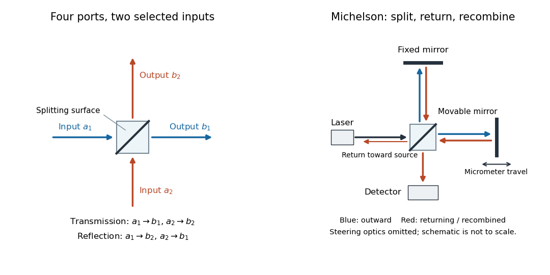
The useful surprise is that the same component divides power with one input and steers power by wave interference with two inputs. In a Michelson interferometer or Mach-Zehnder interferometer, mirror motion changes relative wave phase, turning a small change in optical path length into a measurable change in output power.

Choose an ideal absorbing chemical species with $\epsilon =8000\mathrm{L}\mathrm{mo}{\mathrm{l}}^{-1}\mathrm{c}{\mathrm{m}}^{-1}$ at a fixed wavelength, and a cuvette with geometric length $l=1\mathrm{cm}$. These are stipulated model parameters. A micromolar molar concentration is $1\mu \mathrm{M}=10^{-6}\mathrm{mol}{\mathrm{L}}^{-1}$, so each additional $25\mu \mathrm{M}$ gives $\Delta A=8000\times 1\times 25\times 10^{-6}=0.2$. Five chosen standards therefore predictThe absorbance graph is a straight line of slope $0.008(\mu \mathrm{M}{)}^{-1}$, while the transmittance graph shows exponential decay. Equal increments of molar concentration multiply transmittance by $10^{-0.2}\approx 0.63096$; they do not subtract a fixed transmitted fraction.

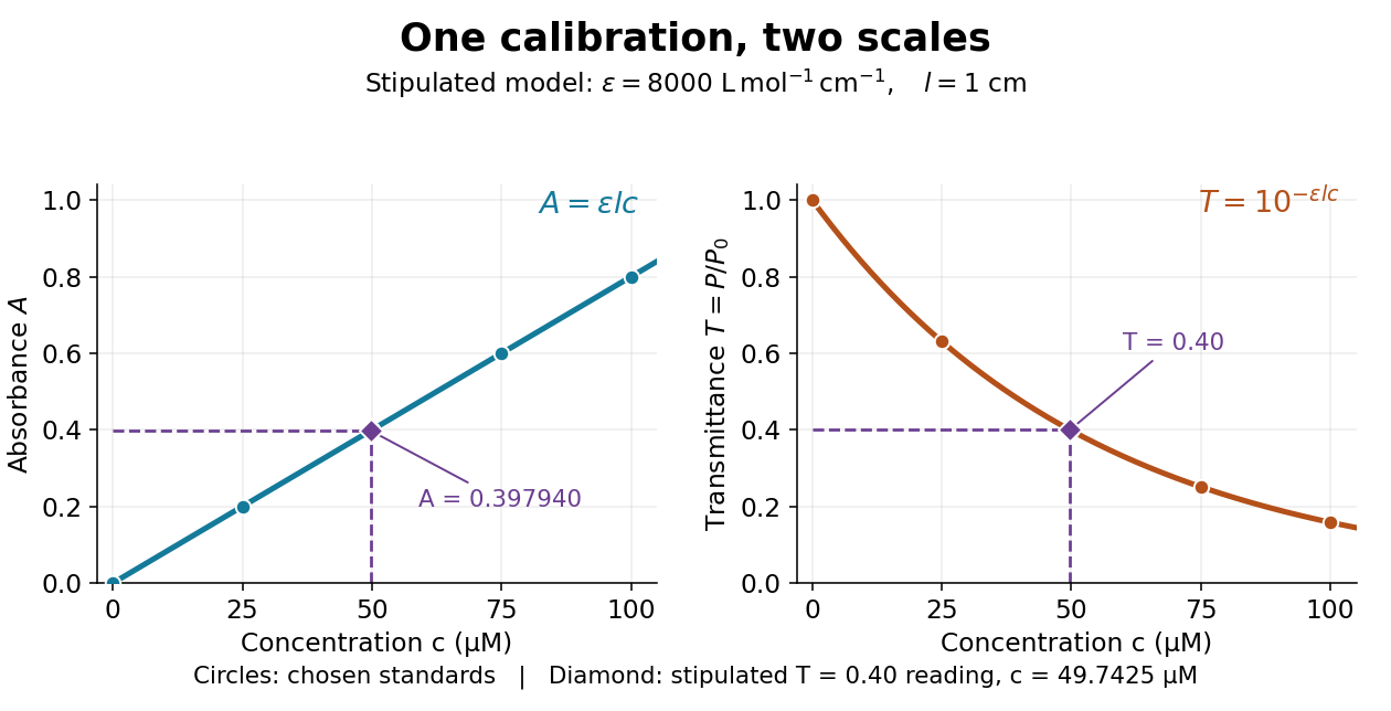
Suppose a measurement returns the stipulated blank-normalized reading $T=0.40$ under those same conditions. The inferred absorbance and molar concentration areThis lies slightly below the $50\mu \mathrm{M}$ standard because $0.40$ is slightly above $10^{-0.4}\approx 0.39811$. A calibration determined experimentally by linear regression may instead have $A=mc+b$. Then use $c=(A-b)/m$, keeping the slope $m$ and intercept $b$ in their measured units. A nonzero intercept calls for checking the reference blank and sample preparation; it does not uniquely identify the cause.

The Beer-Lambert law relates absorbance $A$ to an absorbing species' concentration $c$ and path length $l$ by $A=\epsilon lc$ in a homogeneous medium using sufficiently narrow-band light. The coefficient $\epsilon$ depends on the species, wavelength and chemical solution conditions. This makes Ellman's reagent useful for quantitative thiol assays once its released colored species has been calibrated. ^[ref]

Here $c$ is molar concentration, $l$ is the geometric length through the sample, and $\epsilon$ is the molar absorption coefficient. The ideal beam has parallel light rays, a single wavelength, and a medium with uniform composition and isotropy; finite spectral width must be small relative to features in the optical spectrum.^[ref]

For a spectrophotometer, distinguish the source's output from the reference that reaches the photodetector. Let $P_0$ be the received radiant power through a reference blank and $P$ the received radiant power through the sample, after subtracting the photodetector's dark response. Both refer to the same selected wavelength band and collection geometry. Define the blank-normalized transmittance and absorbance byThe reference blank includes the solvent and other assay ingredients except the absorbing target. Matching cuvettes and conditions makes their common losses divide out. Thus this $T$ is relative to the reference blank; it is not the absolute transmittance of the entire cuvette and its contents. Both radiant powers can be expressed in watts, while their ratio, $T$, and its logarithm, $A$, are dimensionless. An instrument displaying $40\%$ transmission means $T=0.40$, not $T=40$.

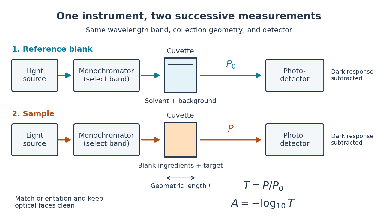
Why take a logarithm? Consider two consecutive identical absorbing layers. Each transmits a fraction $t$ of the radiant power entering it, so together they transmit $t^2$. Their absorbances add because $-{\log }_{10}(t^2)=2(-{\log }_{10}t)$. Doubling the sample length doubles absorbance while squaring transmittance. This turns multiplicative loss into an additive scale and makes a straight line useful for inferring molar concentration.

A short model derivation makes the assumption explicit. Suppose a thin layer of thickness $dx$ removes the fraction $kcdx$ of its incoming radiant power, where $k$ is a fixed constant of proportionality and $c$ is a uniform molar concentration. The corresponding ordinary differential equation, initial condition, and solution areTaking the base-ten logarithm gives $A=kcl/\ln 10$, so $\epsilon =k/\ln 10$. The exponential decay follows from equal layers removing equal fractions of what remains. Proportionality to molar concentration additionally assumes that the absorbing chemical species retains the same response as its molar concentration changes; the geometric argument alone does not establish that.

An actual teaching experiment prepares a Kool-Aid stock by weighing powder, transferring it quantitatively into a volumetric flask, and filling to the mark with water. A Genesys 30 spectrophotometer, blanked with water in a cuvette, scans for the peak absorbance wavelength. A Genesys 10 then measures absorbance at that wavelength, with a water reference blank. Each serial dilution transfers $50\mathrm{mL}$ of the preceding chemical solution to a $100\mathrm{mL}$ volumetric flask and fills to the mark; the protocol records the blank and sample readouts and repeats the halving sequence. These are prescribed experimental steps, not a published numerical data set.^[ref]

The experiment tests whether absorbance tracks the prepared concentration. Its concentration is powder mass per final volume, so the calibration does not by itself supply a single dye's molar absorption coefficient. The manual identifies loss of discrimination for very concentrated, very dilute, or very similar samples.^[ref]

To interpret such a calibration, hold cuvette orientation fixed with its clear faces in the light path, keep fingerprints and bubbles out of that path, and keep the geometric length unchanged. Mix each dilution completely. Re-read the reference blank during the sequence and re-read one standard to test drift. A separate preparation of a standard checks errors propagated through serial dilution; repeating only its instrumental reading does not test the transferred volumes. These controls follow from keeping $P_0$, $l$, and $c$ comparable between readings.

Three mechanisms explain why a straight line can fail. First, scattering of light can divert radiant power away from the photodetector, so cloudiness can raise apparent absorbance without the intended absorbing solute. A reference blank removes only losses shared with the sample. Second, stray light reaching the photodetector can make a strongly absorbing sample appear too transmissive. In an original model with extra detected radiant power $s{P}_0$ in both readings,As the ideal transmittance approaches zero, the reported absorbance approaches ${\log }_{10}((1+s)/s)$ for $s>0$. This finite ceiling is a model prediction, not measured instrument performance.

Third, chemical equilibrium can redistribute the absorbing chemical species when dilution, pH, or temperature changes. Even if each chemical species separately follows the Beer-Lambert law, their combined absorbance is $A=l{\sum }_i{\epsilon }_i{c}_i$, where $c_i$ is each species' molar concentration; changing those fractions need not preserve one effective molar absorption coefficient. Thus an unknown should be compared with standards under matching chemical solution conditions, within the tested concentration range. A good linear regression alone does not establish chemical selectivity.

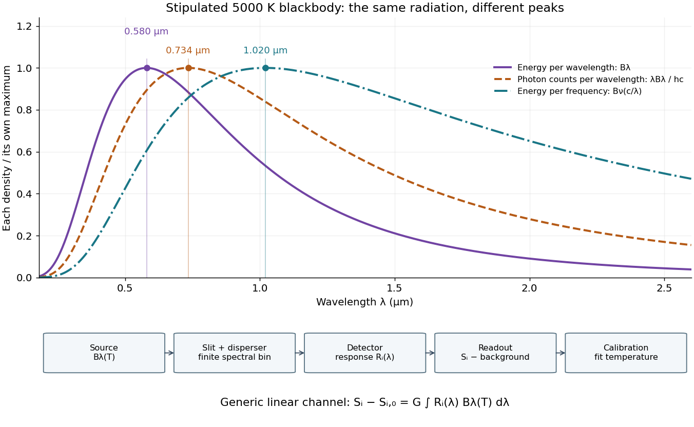
Consider a hypothetical star whose emitted specific intensity is exactly that of a uniform $5000\mathrm{K}$ blackbody. Assume transparent propagation with negligible Doppler shift and interstellar extinction, so geometric dilution multiplies every spectral interval by the same factor. The stipulated temperature givesUsing the converted frequency peak as though it maximized $B_{\lambda }$ would return $b/(c/{\nu }_{\max })\simeq 2841.26\mathrm{K}$, a substantial error caused solely by mixing spectral conventions.

Now stipulate a photodetector with constant quantum efficiency $\eta$ over the relevant wavelengths, collecting equal narrow wavelength bins. For fixed accepted projected area times solid angle $G$, with dilution included in $G$, its expected photon count rate density isThis follows by dividing the received power by the photon energy $hc/\lambda$. It peaks where $x=4(1-e^{-x})$, at $x=3.9206903949\dots$, giving $0.73394057\mu \mathrm{m}$ for the same model star. Constant quantum efficiency is not constant energy spectral responsivity: the latter includes the wavelength-dependent photon energy conversion. For example, $G=10^{-12}{\mathrm{m}}^2\mathrm{sr}$, $\eta =0.5$ and a $1\mathrm{nm}$ bin centered at $0.600\mu \mathrm{m}$ give approximately $1.93\times 10^{10}$ detected photons per second in the narrow-bin approximation. These are calculated model values, not observations of a named star.

A more general linear detector channel has outputwhere $S_{i,0}$ is the background reading and $R_i$ includes spectral selection, optical transmission and detector spectral responsivity. A raw channel maximum need not locate either Planck function maximum. Recovering a temperature requires an appropriate calibrated response and an emission model. For a real stellar atmosphere, opacity and radiative transfer can reshape the spectrum; interstellar extinction can reshape it again. A single peak does not establish a unique physical temperature without those assumptions.