Topics (384k) Articles (398k) Users (410) Discussions (242) Comments (383) Files (13k) New article

Gaussian pulse-width deconvolution uncertainty is the uncertainty in an inferred pulse duration after subtracting a characterized Gaussian instrument contribution. For the Gaussian instrument broadening in third-order pulse correlation model, let be measured correlation full width at half maximum, the additional response width and the inferred pulse width:These widths must use the same convention. The relation already includes the ideal nonlinear gate; represents an additional response.
First-order propagation uses the sensitivity coefficientsThus the standard uncertainty obeysThe negative covariance term follows from the subtraction, not a rule that uncertainties should simply be subtracted. The GUM's general law retains covariance and requires considering higher-order terms when nonlinearity is significant.[ref]
Guide to the expression of uncertainty in measurement by JCGM. §§5.1.2–5.1.3 and 5.2, sensitivity coefficients, nonlinear limitation and correlated inputs
For an original example, and give . With independent , the formula gives . If instead the two width estimates have correlation coefficient 0.8 with those same uncertainties, the covariance is and . The assumed relationship between the estimates changes the result.
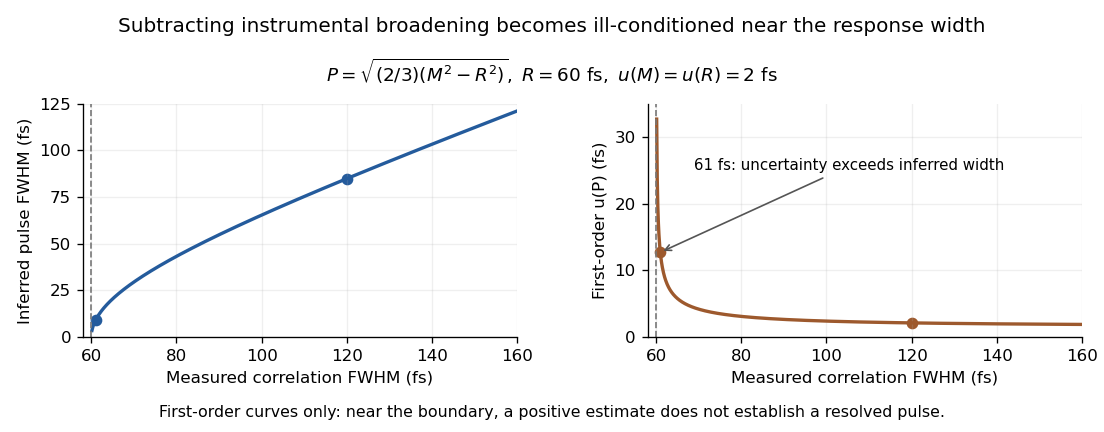
Original Gaussian pulse-width inversion and first-order uncertainty curves for a 60 fs response and independent 2 fs width uncertainties
. Details. Near , both derivatives grow because approaches zero. With , and independent 2 fs uncertainties, the central inferred value is only about while the first-order uncertainty is about . This is an unresolved Gaussian pulse-width estimate under these measurement conditions, rather than a reliably resolved 9 fs pulse.
The quantity being subtracted is , with approximate variance . If plausible width values include , linear symmetric error bars on can be misleading. Report the response assumptions and consider an appropriate nonlinear inference or bound; simply discarding negative radicands would silently change the statistical model. Even a precise inversion remains conditional on the Gaussian response model being physically appropriate.
The floating-pinion compression margin is the amount of relative approach remaining before the less compressed contact reaches zero compression in a stated two-contact model. It turns the assumptions of a floating-pinion balancing mode into a quantitative admissibility check.
For and , let equilibrium position be and defineA positive means both contacts are compressed at equilibrium. If with , then guarantees compression throughout the bounded motion. For a steady single sinusoid and fixed , this is the exact full-cycle condition; a general transient envelope supplies only a sufficient bound.
An original nominal example has and , giving . A displacement amplitude passes that nominal check, leaving of minimum compression for the sinusoidal model.
A floating-pinion robust contact margin includes bounded parameter uncertainty. If and , a conservative lower margin isFor and , . The same amplitude is no longer guaranteed admissible, although failure of the bound does not prove contact loss. Amplitude leaves at least under these independent interval bounds.
In the symmetric static model, givesfor positive mesh stiffness and nonnegative floating-pinion centering stiffness . Mounting freedom can change the margin, but it also changes dynamics; maximizing this one scalar is not a complete gearbox design rule.
A floating-pinion contact-loss check must recompute the contact model once a force reaches zero. The historical face-gear tests provide evidence about mounting freedom and measured torque division under slow rolling, rather than a universal dynamic margin.[ref]
Development of Face Gear Technology for Industrial and Aerospace Power Transmission by Gregory F. Heath and others. Introduction, printed pp. 1–2; Conclusions, printed p. 84
Step-size stability of a reference perturbation checks whether a numerical reference-response estimate behaves consistently as the applied step changes. For a final comparison , a central slope isFor sufficiently smooth , its leading truncation error is proportional to . Comparing several steps tests that numerical behavior, while choosing steps near the physical reference uncertainty also probes whether a local derivative adequately represents the measurement model.[ref]
Guide to the expression of uncertainty in measurement by JCGM. §§5.1.2–5.1.4, nonlinear propagation and sensitivity coefficients
For an original model, let and , with . For , the central slopes are0.210,0.2025 and0.200625. Their successive departures from0.2 shrink by four as halves. Richardson extrapolation removes the cubic contribution exactly in this model:For a general smooth response, it removes the leading term rather than proving exact cancellation of every nonlinear contribution.
Small steps also amplify output error. If each evaluation has absolute error at most , the error in the central slope is at most . With , this bound is at but0.1 at . The cubic truncation term decreases with , whereas this evaluation-error bound increases. Equating their orders, , suggests the scale , here0.001mm. This scale follows from the stipulated error model, not a universal finite-difference setting.
An unchanging central value is also insufficient to establish differentiability. For , every is zero, while the forward and backward slopes are and . Inspecting both one-sided changes reveals the cusp. Likewise, a stable local slope does not rule out a quadratic finite-range response, as finite-perturbation reference sensitivity shows.
A meaningful test changes one assigned shared reference consistently in every dependent calculation, holds the other inputs and computational settings fixed, and records the steps, units, slopes and one-sided changes. Shared reference uncertainty and comparison-process variability are distinct physical contributions in the NIST uncertainty budget.[ref] If evaluation includes simulation noise, separate its repeatability from the response to the changed reference.
Etalon reference-plane dependence is the change in the assigned propagation and reflection phases when the mathematical planes defining an etalon's field amplitudes are moved. A consistently computed etalon round-trip phase and its resonance frequencies remain unchanged. The decomposition into spacer delay and etalon coating group delay depends on those planes.
Use time dependence and a lossless uniform spacer with wavenumber . Let the physical interfaces be separated by , with internal reflection coefficients referred to their surfaces. The round-trip multiplier isThe multilayer formalism explicitly assigns forward and backward amplitudes at specified interfaces and propagates their phases through each layer. Its sign conventions must remain consistent when comparing reflection phases.[ref]
Multilayer optical calculations by Steven J. Byrnes. §4.1, interface amplitudes and propagation; Appendix A, reflection-amplitude conventions
Move the left mathematical reference plane a distance into the spacer, leaving the actual coating in place. A wave launched from that plane travels to the coating and back, so the effective left reflection coefficient becomes . The explicit remaining distance is . HenceThis original derivation changes the representation, not the physical cavity. Moving a real mirror would instead change the system.
Let , using continuous wave phase. Since , the new assigned terms obeyTheir sum equals . If the spacer is dispersive, the corresponding second-derivative contributions likewise transfer between the two terms; the total group delay dispersion is unchanged.
For an original example, take and . The assigned reflection delay increases by about while the assigned propagation delay decreases by the same amount. The free spectral range cannot reveal a change of bookkeeping. An apparent discrepancy of that size between two coating calculations can arise solely from different reference planes.
Report the incident medium, polarization, reference surfaces and phase convention with a coating-delay result. A measured resonance spectrum constrains the total phase; independently identifying a coating contribution requires a compatible spacer model. Etalon delay inferred from free spectral range therefore should not be compared with an isolated coating derivative until both calculations use the same reference planes.
A clearance certificate with bounded distance-query error proves separation over a continuous motion interval when sampled distances are known only within stated error bounds. A positive returned value from collision detection is not by itself a lower bound on the true geometric distance. Approximation, floating-point error and model error must be included if they affect the intended claim.
Let true set distance satisfy on . At endpoints, assume certified query errors . DefineProvided the query bounds are consistent with nonnegative distances, . The endpoint lower bounds propagate intoThis extends the endpoint certificate for continuous collision clearance. The primary planning model requires feasibility along the whole continuous path; checking endpoint poses alone is insufficient.[ref]
Robotic Systems by Kris Hauser. Chapter 8, Point-to-point path planning; Chapter 9, rotational configuration-space obstacles
The minimum of this envelope must be computed on the actual interval. Its general closed form, including unequal lower bounds, isFor and , the two sloping bounds meet inside the interval and the average expression dominates the other nonzero candidates. If , their intersection lies before the interval; the minimum is instead . The opposite inequality exchanges the endpoints. For , the formula reduces to because true clearance is constant.
The lower bounds themselves need not satisfy the consistency condition for exact endpoint distances. For example, , and permit a true clearance rising from to . Rejecting these lower bounds because their difference exceeds would wrongly treat them as exact observations. The general certificate gives ; using only the intersecting-cone expression would give the weaker .
A second original example takes reported distances and , errors and , and . Then and , so . The error-free formula would have claimed . For a required strict margin above , the uncertain queries do not certify the interval. Tightening both errors to raises the lower bound to and supplies the requested certificate.
Compatibility of bounded endpoint distance queries also uses the upper bounds. The intervals must obey , , and . A violated condition signals inconsistent assumptions. An upper distance bound at or below a required margin can establish a sampled margin violation; failure of a lower-bound certificate alone does not establish a collision.
A proposed checker records the query’s enclosure guarantee, units and geometric model, propagates the motion bound with the actual interpolation, and leaves uncertified intervals unresolved for further subdivision or stronger queries. A standard deviation is not a deterministic query enclosure. A certificate against a nominal obstacle model also needs a separate justified relation to the actual obstacle geometry before it can be interpreted physically.
The beam shear correction coefficient adjusts a reduced beam model's shear response for the nonuniform shear stress over a material section. With shear modulus , area , transverse force resultant and generalized beam shear angle ,where is effective beam shear rigidity. Bower's primary account calls this the Timoshenko shear coefficient and explains that its value depends on geometry, Poisson's ratio and how the approximate theory is matched to the underlying solid.[ref]
Applied Mechanics of Solids by A. F. Bower. §8.7.2, Timoshenko force relation and following shear-coefficient paragraph
An original energy-matching derivation makes the correction precise for one approximation. Assume uniform and a chosen shear-stress field with resultant . The shear elastic energy per unit beam length and its reduced representation areThusThe Cauchy-Schwarz inequality gives , hence for this definition. Equality requires uniform stress. This bound belongs to the stated energy-matching definition rather than every convention called a shear correction coefficient.
For the parabolic rectangular stress approximation used in effective beam shear rigidity, the squared-stress integral is , giving . Choose , and . Then and radians. Omitting the correction gives , underestimating this generalized shear angle by one sixth.
The generalized angle also differs from the peak local shear strain. Under the same parabolic approximation, peak stress is , giving peak strain . The values describe different reductions of the same chosen stress field. Identifying from a bending test therefore requires the section model and displacement readout, not merely a material modulus. For a three-point bending test, the shear deflection contribution varies as , whereas bending varies as ; a span comparison can help separate them.
A snake is a member of an elongated, predominantly limbless reptile lineage within Squamata. Limb reduction is one feature of its evolutionary history, not evidence that the lineage has no relationship to limbed ancestors. Different snakes retain different remnants of the ancestral limb-development system.
A study of a limb regulatory enhancer found progressive functional loss in snake sequences. Replacing the corresponding enhancer in mice with a snake-derived sequence produced severe limb reduction, linking a regulatory DNA change to developmental output. [ref]
Progressive Loss of Function in a Limb Enhancer during Snake Evolution by Evgeny Z. Kvon and others. 2016, abstract and genomic enhancer-replacement experiments
This identifies a contributing mechanism; it does not show that one sequence change alone explains every anatomical specialization of snakes.The de Rham complex of a smooth manifold is the cochain complex of smooth differential forms with exterior derivative:Here and . The identity makes every exact differential form closed. The quotient of closed -forms by exact -forms is the de Rham cohomology group .[ref]
Introduction to Smooth Manifolds, second edition by John M. Lee. Chapters 14 and 17, exterior differentiation and de Rham cohomology
In Euclidean space the Poincaré lemma makes this complex exact in positive degrees. On a general manifold it is locally exact in small coordinate balls, but global exactness can fail. For the unit circle, the restriction of has integral around one positive turn. It is closed, since the circle has no nonzero two-forms. It cannot equal for a globally defined smooth function on the circle: the integral of a derivative around a closed loop is zero.
A signed-filter current-sign certificate guarantees the sign of an actual load current from a filtered estimate whose coefficients can be negative. Such a filter may extrapolate or sharpen a waveform, but its output is not necessarily a convex average of past currents. The sign must hold over the intended switching interval before it can justify current-polarity dead-time compensation; the relevant recirculation paths depend on current direction.[ref]
Suppose , with , and the Lipschitz bound over all relevant times. ThenThe absolute coefficients are essential. To certify an interval, maximize the right-hand side over its times. A positive sign follows if the estimate exceeds that bound; a negative sign follows if it is less than the negative bound. If individual sample errors are bounded by , their contribution is at most rather than a signed cancellation.
The generic bound can be conservative because all samples come from the same current history. For the two-tap predictor and future time , rewrite the error asThis gives the sharper resultinstead of the direct absolute-weight bound . It is sharp under only a Lipschitz current assumption: a history proportional to changes slope at the central sample and attains the positive error limit. The Lipschitz assumption permits that corner even though a derivative need not exist at the corner itself.
For an original example, take , , a target interval , and aggregate estimate error . The sharper interval bound is ; the direct absolute-weight bound is . A reading therefore certifies at least throughout the interval using the sharper proof. A signed timestamp average would misleadingly place the predictor at time ; it is an extrapolation, not a measured future sample.
A current-sign certificate with a curvature bound can exploit stronger information. For the target time and a twice differentiable current with on ,Taylor’s theorem, or integrating the second derivative against its triangular weight, proves the inequality. At and stipulated , the model error bound is before sample errors. This smaller number is justified only if the curvature bound also covers switching transitions; an affine-ramp fit alone does not establish it.
A proposed validation injects known ramps and waveforms with changing slope, records the actual filter coefficients and sampling times, and checks the resulting enclosures against an independent current trace. Account for sensor saturation, timing uncertainty and the history used by the filter. A sharper mathematical bound and a stronger physical assumption are different ways of obtaining a smaller certificate margin.
The relation between current distortion factor and THD with DC current accounts for the mean component omitted from the usual fundamental-normalized total harmonic distortion. For a periodic electric current, let be its signed DC component, the fundamental RMS magnitude, and the RMS magnitudes of higher harmonic components. The Parseval identity givesDefine and current distortion factor . Division by provesThe root mean square in this expression includes the mean, while the stated total harmonic distortion excludes it. An instrument reporting AC-only RMS or a differently normalized distortion quantity requires a correspondingly different conversion.
For an original example, take , and combined higher-harmonic RMS magnitude . Then , and . Neglecting the DC component would instead predict . In the same conductor electrical resistance , the actual heating is , while that omission would predict .
For a zero-mean sinusoidal supply of RMS and an in-phase fundamental current, the example absorbs . Its apparent power is approximately , so total power factor is despite a displacement power factor of one. The DC component carries no average power from that particular zero-mean supply, but it still increases mean-square electric current. If the supply itself has a DC component, its contribution must be included through the harmonic active power sum.
As tends to zero the defining current distortion factor can tend to zero, but fundamental-normalized total harmonic distortion is undefined at . Do not evaluate the boxed relation there by silently dividing by zero. The manufacturer's documentation also uses differing labels for distortion ratios, reinforcing the need to state the defining normalization.[ref][ref]
Overview of Functions: Harmonic Measurements by Schneider Electric. Quality Indicators, Distortion Factor
Contact-mode timestep stability concerns whether a numerical integrator introduces growing errors when advancing the fast dynamics of an active penalty contact. It depends on the integration rule and the local modal frequencies, not just the size of the modeled overlap. The primary compliant-contact treatment identifies stiff contact springs as a source of numerically stiff differential equations.[ref]
Underactuated Robotics by Russ Tedrake. Multi-Body Dynamics, Compliant Contact Models, stiff-spring and numerical integration discussion
Freeze the active contacts and linearize about a compressed equilibrium. An undamped mode has . For step , put . The Forward Euler method updates displacement and velocity with matrixwhose eigenvalues are . Their magnitudes are whenever . Thus the method has no nonzero stable step for indefinite integration of this undamped oscillator, although smaller steps reduce its error on a fixed finite interval.
The central-difference recurrence instead givesFor its two distinct amplification roots lie on the unit circle. At the repeated root is , and solutions can include , so the strict bound matters. A collection of frozen undamped modes therefore requires for this oscillatory stability condition. In coupled normal-contact penalty modes, comes from the coupled system rather than an arbitrary total-mass estimate.
Stability still allows substantial contact-mode numerical phase error. For central differences the phase per step is , giving numerical angular frequency . At and , is stable but the numerical frequency is about , high. A timing-sensitive contact event can consequently drift even when oscillation amplitudes do not grow.
Implicit schemes illustrate another tradeoff. For the Backward Euler method, the amplification factors are and have magnitude . At , each step reduces the oscillatory amplitude by about , despite the continuous undamped system conserving energy. The trapezoidal rule instead has factorswith phase . The same example gives , low. Unconditional stability for this linear model does not imply correct timing at a large step.
A practical error check therefore compares both amplitude and phase while reducing . For instance, a small target dimensionless step gives much smaller phase error than one, but the acceptable value depends on the observable and time span; it is not a universal accuracy certificate.
The frozen-mode argument has a defined scope. Contact opening changes the active stiffness, nonlinear force laws change tangent stiffness, and damping introduces additional eigenvalue scales. An integrator can satisfy the local oscillator bound while missing an intervening collision or contact release. A proposed test starts with a small compressed-contact perturbation, checks frequencies and energy behavior, then repeats across a known contact-opening event with decreasing steps. Record force histories and event times as well as penetration, so numerical damping or phase drift is not mistaken for a material response.
A pointwise convolution uses a spatial kernel of size one to combine neural network channels independently at each spatial position. For a two-dimensional input this is a one-by-one convolutional layer. In the ordinary dense-channel, unit-stride case, the same affine map acts on the channel vector at every grid point.[ref]
Conv2d in the PyTorch documentation. Opening equation and kernel_size/stride parameters, specialized to kernel size one and groups=1
Let be the channel vector at position . With weight matrix and neural network bias vector , the output isThis is matrix multiplication across channels, not an average of neighboring spatial positions. The same and are reused throughout the grid.
For an example without biases, takeAt a point with input the output is . At another point with input it is . A three-channel neural network feature map has become a two-channel map without mixing the two positions.
There are weights, plus optional biases. Thus three input and two output channels require six weights, or eight parameters including biases. A dense three-by-three filter with the same channel counts requires weights, or fifty-six parameters with biases. This comparison counts parameters for the stated connectivity; it does not claim that the two layers compute equivalent functions.
Channel reduction can make a later spatial convolutional layer cheaper. The original Inception uses one-by-one reductions before some larger filters. A pointwise operation can also increase the channel count; size one refers to its spatial footprint, not to the number of channels.[ref]
Going Deeper with Convolutions by Christian Szegedy and others. §4 and Fig. 2, one-by-one dimension-reduction branches
With no intervening spatial operation, pointwise layers and pointwise activation functions alone do not enlarge the spatial neural network receptive field.The convolution stride specifies how far the filter's origin advances between neighboring output positions of a convolutional layer. It controls which spatial positions are evaluated. A larger stride usually produces a smaller output grid without changing the number of coefficients in each filter.[ref]
For a real one-dimensional example, take the inputand a size-three all-ones filter, no bias and no padding. Using the unflipped cross-correlation convention, stride one evaluates windows beginning at indices and givesStride two evaluates windows beginning at indices , givingThe second result keeps every second origin from this first grid; it still combines three input values for each retained origin.
For an undilated length- input and length- filter, no padding and stride , a zero-indexed output uses input indices through . Requiring its last index not to exceed gives . Counting the admissible nonnegative integers therefore giveswhen and is a positive integer. The floor function is essential when the last candidate origin would extend beyond the input.
With symmetric zero padding of positions per side and convolution dilation , the corresponding standard shape expression isHere dilation changes the spacing of samples within a filter footprint; stride changes the spacing between filter origins. The two parameters have different roles.[ref]
Conv2d in the PyTorch documentation. Parameters, stride/padding/dilation; Shape, each spatial-axis formula
For two-dimensional data, specify a stride for each spatial axis; unequal strides need not reduce height and width by the same amount. The weights of the filter remain shared across the visited positions. Stride also changes how neighboring outputs' neural network receptive fields are spaced in the original input, so it affects more than just a displayed array size.
Convolution dilation specifies the spacing between neighboring kernel sample points in a convolutional layer. Dilation one samples adjacent positions; larger dilation separates those positions while keeping the filter's learned coefficient count fixed. Convolution stride instead controls the spacing between successive filter origins.[ref]
Conv2d in the PyTorch documentation. Opening parameter descriptions; Parameters, dilation and stride
For an own real one-dimensional example, takeand coefficients , with stride one, no padding and no bias. Use the unflipped cross-correlation convention. Dilation one sums three adjacent values and gives . Dilation two instead uses offsets :The second filter evaluates a wider input span while still using three coefficients.
For sampled coefficients separated by positions, the first-to-last displacement is . Including the first position gives the effective convolution kernel sizeThus spans five positions. At each origin only three of those five positions are sampled directly.
The same linear operation can be represented by a dense width-five kernel . The inserted zeros are fixed structure, not additional trainable coefficients. Dilation changes the footprint without making the original three-parameter filter a general five-parameter one.[ref]
Conv2d in the PyTorch documentation. Variables, weight shape depends on kernel dimensions and channel connectivity
For input length , symmetric zero padding and stride , the usual per-axis size formula becomeswhen the padded input accommodates the footprint. The example gives outputs. The floor function counts origins whose final sample remains in range.[ref]
Dilation can enlarge a unit's spatial neural network receptive field without evaluating every intervening input position. Whether later layers fill those gaps depends on the architecture. A wider span alone does not establish greater numerical influence at every position or better performance on a learning task.
A one-sided Cantelli confidence bound with a bias budget combines a validated bound on the estimator's systematic displacement with a one-sided variance inequality. Suppose , where is deterministic, and a nonnegative statistic satisfies almost surely. For , defineThen . This is a lower confidence bound, with an unbounded upper side.
For the proof, put . If , the bias bound impliesFor positive , Cantelli's inequality bounds this event by at the last displayed threshold . For zero variance, almost surely and the conclusion follows directly. A random may depend on the centre: the samplewise comparison is what supports the event inclusion.
For an original numerical bound, let , , , and . The square-root term is , so is a 90 percent lower bound under these assumptions. Reversing the inequality gives the separately valid upper bound . Each has 90 percent one-sided coverage; reporting both endpoints together only guarantees 80 percent by the union bound. To guarantee a joint 90 percent interval this way, allocate error probabilities summing to across its two sides.
This construction complements the two-sided result in confidence bounds from a samplewise variance bound. It needs a bias bound and an almost-sure variance bound, not merely a conservative variance estimator in the expected-value sense. A coverage interpretation must follow the actual tail argument, as emphasized by NIST's discussion of expanded uncertainty.[ref]
An irreducible complex analytic hypersurface in a complex manifold is a complex analytic hypersurface that cannot be written as the union of two proper closed analytic subsets. It has pure complex codimension one. Irreducibility is a condition on decomposition into analytic pieces, rather than a requirement of smoothness.
In , the hypersurface is reducible: it is the union of the two coordinate axes. The cusp is irreducible but singular at the origin. Its equation is irreducible as a convergent germ of a holomorphic function there, while both first derivatives of vanish at zero. Thus irreducibility does not force the holomorphic implicit function theorem to apply.
Global irreducibility and irreducibility of every local germ must be distinguished in general. Local factorization of a reduced defining equation records its analytic branches, while global irreducibility concerns a decomposition of the entire hypersurface. Such hypersurfaces provide the prime components used to describe complex analytic divisors.
The gain-matching condition for heterodyne normalization is the relation between three positive multiplicative calibration factors that leaves a normalized beat unchanged. If the corrected peak beat current is and the separate arm currents are , thenExact cancellation therefore requires , or equivalentlyThe beat-channel gain must equal the geometric mean of the arm-channel gains. The three gains need not individually agree.
An original example uses and . Their geometric mean is 0.99, so gives exact cancellation. Keeping instead multiplies the inferred overlap by . Choosing the arithmetic mean 1.01 for would not solve the problem: it would multiply the result by approximately 1.02020. These are stipulated calibration factors, not receiver specifications.
For time-dependent gains, the condition must hold for the corresponding measurements in each realization if sample-by-sample invariance is claimed. Merely arranging zero mean logarithmic mismatch does not guarantee an unbiased arithmetic overlap: lognormal bias of a heterodyne overlap estimate gives a counterexample under Gaussian log-errors.
A heterodyne RF-to-DC gain transfer check distinguishes electronic amplification in the beat-frequency path from the response used for the arm currents. A change confined to does not cancel. Neither does a generic additive dark-current error satisfy this multiplicative model. Preserve the amplitude convention as well: is a corrected peak current, rather than the unconverted electrical beat power.
The NIST receiver experiment used two lasers, a beam splitter, a polarizer and single-mode collection to establish optical matching, while separately correcting the electrical measurement path.[ref]
Frequency response metrology for high-speed optical receivers by Paul D. Hale and others. PDF pp. 1–2, Heterodyne measurements and Eqs. 1–4
Those different physical operations explain why one common scalar gain is a special case rather than an automatic description of the entire apparatus.One practical test varies a suspected common gain while holding powers, mode matching and collection conditions fixed, and checks whether the normalized result stays constant. Passing that test constrains response to that change; it does not exclude an unchanged systematic mismatch. Report the gain-sharing model and the remaining uncertainty before interpreting normalization as complete calibration cancellation.
Lognormal bias of a heterodyne overlap estimate is the upward mean shift that remains when a zero-mean Gaussian logarithmic error is exponentiated. It does not undo common-gain cancellation in heterodyne overlap uncertainty: a perfectly shared gain cancels in every reading, while residual mismatched gains can still fluctuate.
Write the normalized positive estimate as , with fixed true overlap magnitude and . The moment-generating function of the normal distribution givesThese are exact lognormal distribution identities under the stated error model. When , the logarithmic estimate is centered correctly and the median is , but the arithmetic mean exceeds it by relative amount .
For an original deliberately visible example, and logarithmic standard deviation 0.2 give and mean about 0.81616: a 2.02% mean shift. The values are chosen statistical parameters, not uncertainties reported for a receiver. An estimate can also exceed the physical consistency bound for separately measured heterodyne arm powers; the noisy readout is not itself a physical overlap above one.
If and are known, multiplying the estimate by corrects its mean in this model. Uncertain variance in heterodyne lognormal bias correction matters when those parameters are estimated: plugging in a noisy variance, especially from related data, is not automatically an exact correction.
Averaging logarithms has a different interpretation from averaging overlaps. For independent zero-mean log-errors of variance , the geometric mean is , whose arithmetic expectation is . A gain component shared across the entire run does not acquire the independent-shot variance reduction.
The physical calibration paths determine the logarithmic covariance. NIST's heterodyne apparatus controlled the optical modes while separately correcting electrical loss and impedance mismatch.[ref]
Frequency response metrology for high-speed optical receivers by Paul D. Hale and others. PDF pp. 1–2, Heterodyne measurements and Eqs. 1–4
A first-order uncertainty calculation alone is not this exact distributional model; nonlinear effects and correlated inputs must be assessed explicitly.[ref] State the assumed distribution and the intended summary rather than treating median, geometric mean and arithmetic mean as interchangeable.A centripetal amplitude-error budget allocates the permitted error in an oscillating centripetal correction between amplitude mismatch and phase mismatch. If the true correction amplitude is , the applied amplitude is and the relative phase is , phasor subtraction gives residual amplitudeThe first term remains even with perfect timing. The second consumes part of the same acceleration-error budget; their separate limits cannot both be set to the entire allowed residual.
Write . For small and , the leading approximation isThis provides an approximate joint budget, rather than permission to allow the maximum phase error and maximum gain error simultaneously. For an original example, and residual limit give relative budget0.025. Assigning relative amplitude error0.015 leaves an approximate phase budget0.020rad. The exact formula, with , gives a slightly smaller bound of about0.01985rad.
A centripetal speed-gain error illustrates how the mismatch can arise. For , using radius and a speed reading scaled by producesWith correct radius and , the correction is2.01% high. In a small-ripple model whose constant speed and ripple amplitude are both scaled by the same sensor gain, the oscillating correction amplitude has this same gain factor. For that alone gives0.0804m/s² amplitude mismatch. The constant centripetal term also needs its own error check; budgeting only the ripple does not control it.
Rotating-frame components and the rotation reference are experimentally consequential: a primary MEMS-sensor study compares rotating transmission measurements with stationary housing accelerometers and reconstructs a timing reference.[ref]
Evaluation of MEMS-Based Wireless Accelerometer Sensors in Detecting Gear Tooth Faults in Helicopter Transmissions by David G. Lewicki and others. Printed pp.19–21, rotating-frame components; pp.24–25, rotation timing
The budgets above are original illustrative calculations. Actual limits require the relevant operating speeds, radii, frequency range and measurement calibration, alongside the centripetal phase-error tolerance.Individualization-refinement graph search explores possible vertex labelings while repeatedly distinguishing vertices by their adjacency structure. It combines inexpensive colour refinement with branching when refinement leaves indistinguishable vertices. This is a framework for canonical graph labeling and graph automorphism computation, rather than a claim that degree information alone decides graph isomorphism.[ref]
Practical graph isomorphism, II by Brendan D. McKay and Adolfo Piperno. Sections2.3–2.4, search tree and canonical forms; §3.1, refinement
Start with an ordered partition of a set of the vertex set, representing any prescribed vertex colours. Within each cell, compare the number of neighbours each vertex has in every current cell. Split a cell whenever those count vectors differ, and repeat until no further split occurs. The result is an equitable partition. A discrete partition of a set, with one vertex per cell, gives a candidate vertex ordering.
If a cell still has several vertices, choose a target cell by a rule preserved under relabeling. For each possible chosen vertex in that cell, make that vertex a singleton, refine again and continue recursively. The leaves provide candidate encodings of the adjacency matrix. Choosing a fixed extremal encoding over the complete search gives a canonical representative. Implementations use valid node invariants and discovered graph automorphisms to prune branches without changing the result.[ref]
For an original example, label a six-vertex cycle graph temporarily as , with adjacency modulo6. Starting with one cell, every vertex has two neighbours, so colour refinement alone leaves one cell. Individualizing vertex0and refining givesVertices1and5remain indistinguishable because reflection fixing0exchanges them. Individualizing one of them resolves the remaining pairs. The temporary names explain the search; they cannot be used as invariant tie-breakers that silently discard the other possible labeling.
By contrast, two disjoint triangles also begin with six vertices of degree2, but after individualizing one vertex the refined cell sizes are1,2,3. The cycle's sizes are1,2,2,1. Thus this branch detects structure that initial degree refinement misses. Highly symmetric graphs can still require extensive search; refinement is a reduction of the search space, not a universal small bound on it.
Pinned article: Introduction to the OurBigBook Project
Welcome to the OurBigBook Project! Our goal is to create the perfect publishing platform for STEM subjects, and get university-level students to write the best free STEM tutorials ever.
Everyone is welcome to create an account and play with the site: ourbigbook.com/go/register. We belive that students themselves can write amazing tutorials, but teachers are welcome too. You can write about anything you want, it doesn't have to be STEM or even educational. Silly test content is very welcome and you won't be penalized in any way. Just keep it legal!
Intro to OurBigBook
. Source. We have two killer features:
- topics: topics group articles by different users with the same title, e.g. here is the topic for the "Fundamental Theorem of Calculus" ourbigbook.com/go/topic/fundamental-theorem-of-calculusArticles of different users are sorted by upvote within each article page. This feature is a bit like:
- a Wikipedia where each user can have their own version of each article
- a Q&A website like Stack Overflow, where multiple people can give their views on a given topic, and the best ones are sorted by upvote. Except you don't need to wait for someone to ask first, and any topic goes, no matter how narrow or broad
This feature makes it possible for readers to find better explanations of any topic created by other writers. And it allows writers to create an explanation in a place that readers might actually find it.
Figure 1. Screenshot of the "Derivative" topic page. View it live at: ourbigbook.com/go/topic/derivativeVideo 2. OurBigBook Web topics demo. Source. - local editing: you can store all your personal knowledge base content locally in a plaintext markup format that can be edited locally and published either:This way you can be sure that even if OurBigBook.com were to go down one day (which we have no plans to do as it is quite cheap to host!), your content will still be perfectly readable as a static site.
- to OurBigBook.com to get awesome multi-user features like topics and likes
- as HTML files to a static website, which you can host yourself for free on many external providers like GitHub Pages, and remain in full control

Figure 2. You can publish local OurBigBook lightweight markup files to either OurBigBook.com or as a static website.
Figure 3. Visual Studio Code extension installation.
Figure 5. . You can also edit articles on the Web editor without installing anything locally. Video 3. Edit locally and publish demo. Source. This shows editing OurBigBook Markup and publishing it using the Visual Studio Code extension. 
- Infinitely deep tables of contents:



All our software is open source and hosted at: github.com/ourbigbook/ourbigbook
Further documentation can be found at: docs.ourbigbook.com
Feel free to reach our to us for any help or suggestions: docs.ourbigbook.com/#contact